
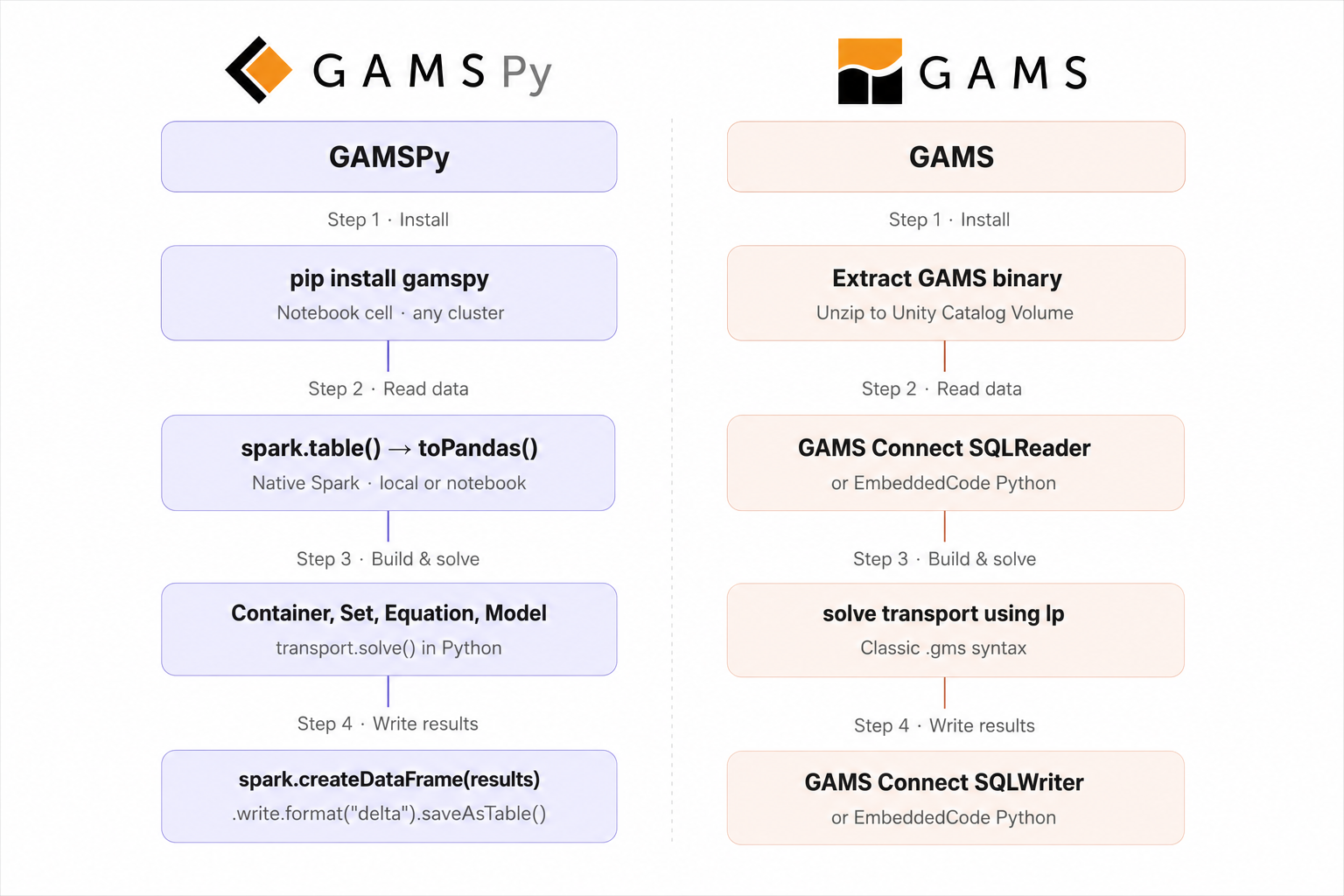
Who this is for
If you are a GAMS user who has migrated to Databricks, or if your organization relies on the Databricks Lakehouse and you need a high-performance tool to embed optimization directly into your data pipelines, this post is for you. Moving data between environments is a relic of the past; with GAMS and GAMSPy, you can formulate and solve large-scale optimization models without ever duplicating data or leaving your secure environment. Databricks has become the central hub for enterprise data-managed in Delta tables, governed by Unity Catalog, and queryable via SQL. While the integration is straightforward, navigating the initial setup can be a hurdle. This walkthrough is designed to clear that path, providing a definitive guide for basic GAMS and GAMSPy use cases in the modern data stack.
Through this step by step tutorial, you will learn to:
- Install GAMS/GAMSPy on your compute
- Streamline data reading from Databricks directly into your models
- Solve a model with GAMS/GAMSPy (Locally or in a Databricks notebook)
- Write the solution back to Delta tables
This tutorial does not aim to cover endless possibilities of using your data with Databricks. It instead focuses on the optimization part of your decision pipeline.
Step 0: Prerequisites
It is assumed that the user is familiar with the basic GAMS/GAMSPy syntax, and has a Databricks account. Depending on where you are trying to read the data into, the connection to Databricks varies slightly. If you are in the Databricks environment such as a notebook, you have spark available readily and you can use it to read data tables. However, if you want to to develop and run models locally and simply use Databricks as the data layer, this needs to be done with Databricks Connect which lets a local Python script use spark as if it were running on the cluster, without any changes to the model code. databricks-connect is pip-installable and your system can be configured with Databricks credentials using databricks configure --token from your terminal. This prompts you for your workspace URL and a personal access token, then writes them to ~/.databrickscfg. Every subsequent script picks this up automatically.
C:\Users\username>databricks configure --token
Databricks workspace host (https://...): <your_host>.databricks.com
Personal access token: ************************************
Once set up, you can create spark explicitly with DatabricksSession. The code-snippets in this blog-post assume that you have appropriately initialized spark depending on your requirement.
# Notebook: spark is provided automatically, no import needed
from databricks.connect import DatabricksSession
spark = DatabricksSession.builder.getOrCreate()
Note that databricks-connect requires an active all-purpose compute resource. To verify the connection is working:
databricks clusters list
Setup used
- Compute: Databricks workspace with a dedicated personal compute cluster (AWS in this case)
- SQL: Databricks Serverless SQL Warehouse, used to create and query Delta tables via the SQL Editor
Demo example
This tutorial uses the classic transport problem. This is a simple LP but it is sufficient to demonstrate the flow of data in a complex decision pipeline consisting of Databricks data and GAMS/GAMSPy model.
Two plants can ship goods to three markets and given all the required data about the demands, supply capacity, and transportation costs, we want to minimize the total transportation cost.

| New York | Chicago | Topeka | |
|---|---|---|---|
| Seattle (cap: 350) | $0.225 | $0.153 | $0.162 |
| San Diego (cap: 600) | $0.225 | $0.162 | $0.126 |
Market demands: New York 325, Chicago 300, Topeka 275.
The formulation
Let $ x_{ij} $ be the number of cases shipped from plant $ i $ to market $ j $.
minimize total shipping cost:
$ \min \sum_{i,j} c_{ij} \cdot x_{ij} $
subject to:
supply constraints: do not exceed plant capacity:
$ \sum_j x_{ij} \leq a_i \quad \forall i $
demand constraints: satisfy each market:
$ \sum_i x_{ij} \geq b_j \quad \forall j $
$ x_{ij} \geq 0 \quad \forall i, j $
It is assumed that all model inputs are Delta tables in Databricks. This reflects how real production models work: your supply, demand, and cost data are already in your Lakehouse, maintained by other pipelines, and your optimization model is a consumer of that data.
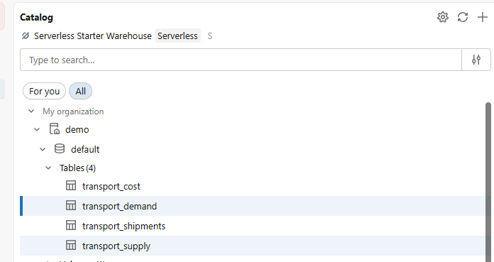
The three input tables for the transport problem are:
demo.default.transport_supply- plant names and available capacitydemo.default.transport_demand- market names and required demanddemo.default.transport_cost- unit shipping cost for each plant-market pair
For this post, we created these using the Databricks SQL editor connected to a Serverless SQL Warehouse. Once run, all four tables (including the empty transport_shipments output table) are visible in the Catalog Explorer.
GAMSPy
Step 1: GAMSPy installation and licensing
GAMSPy needs to be installed on your dedicated compute cluster. Open your Databricks notebook and run:
%pip install gamspy
GAMSPy requires a valid GAMS license to solve models beyond the community edition limits. To add your license on the cluster:
!gamspy install license <access code or path_to_ascii_file>
Step 2: Read data into Python
CATALOG = "demo"
SCHEMA = "default"
def full(table: str) -> str:
return f"{CATALOG}.{SCHEMA}.{table}"
# When running locally
#from databricks.connect import DatabricksSession
#spark = DatabricksSession.builder.getOrCreate()
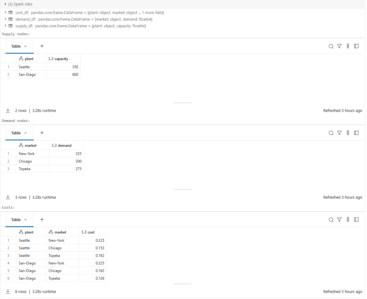
supply_df = spark.table(full("transport_supply")).toPandas()
demand_df = spark.table(full("transport_demand")).toPandas()
cost_df = spark.table(full("transport_cost")).toPandas()
print("Supply nodes:")
display(supply_df)
print("Demand nodes:")
display(demand_df)
print("Costs:")
display(cost_df)
Step 3: Build and solve the model
The model can also be found in the GAMSPy examples GitHub repository.
from gamspy import Container, Set, Parameter, Variable, Equation, Model, Sum, Sense

m = Container()

i = Set(m, name="i", description="supply nodes / plants")
j = Set(m, name="j", description="demand nodes / markets")

a = Parameter(
    m, name="a", domain=[i],
    domain_forwarding=True,
    records=supply_df.rename(columns={"plant": "i", "capacity": "value"}),
    description="plant capacity (cases)"
)

b = Parameter(
    m, name="b", domain=[j],
    domain_forwarding=True,
    records=demand_df.rename(columns={"market": "j", "demand": "value"}),
    description="market demand (cases)"
)

c = Parameter(
    m, name="c", domain=[i, j],
    records=cost_df.rename(columns={"plant": "i", "market": "j", "cost": "value"}),
    description="transport cost ($ per case per 1000 miles)"
)

x = Variable(
    m, name="x", domain=[i, j], type="positive",
    description="shipment quantity (cases)"
)

supply = Equation(m, name="supply", domain=[i], description="do not ship more than available capacity")
supply[i] = Sum(j, x[i, j]) <= a[i]

demand = Equation(m, name="demand", domain=[j], description="satisfy each market's demand")
demand[j] = Sum(i, x[i, j]) >= b[j]

cost_obj = Sum((i, j), c[i, j] * x[i, j])

transport = Model(
    m,
    name="transport",
    equations=m.getEquations(),
    problem="LP",
    sense=Sense.MIN,
    objective=cost_obj,
)

transport.solve()

print(f"\nSolve status : {transport.solve_status}")
print(f"Model status : {transport.status}")
print(f"Objective ($) : {transport.objective_value:.4f}")
Step 4: Write results back
Finally, you can write the shipment quantities back to Databricks as shown below.
from datetime import datetime, timezone

results = x.records.copy()
results.columns = ["plant", "market", "quantity", "marginal", "lower", "upper", "scale"]
results = results[["plant", "market", "quantity"]].query("quantity > 0").reset_index(drop=True)

print("\nOptimal shipment plan:")
print(results.to_string(index=False))

run_ts = datetime.now(timezone.utc)
results["run_ts"] = run_ts


# Note: When running locally, spark is initialized using databricks-connect
result_sdf = spark.createDataFrame(results)

# Overwrite with this run's results (append if you want history)
(result_sdf
    .write
    .format("delta")
    .mode("overwrite")
    .option("overwriteSchema", "true")
    .saveAsTable(full("transport_shipments")))

print(f"\n Shipments written to {full('transport_shipments')} at {run_ts}")
display(spark.table(full("transport_shipments")))
The terminal output is shown below
results
           i         j  level  marginal  lower  upper  scale
0    Seattle  New-York   50.0     0.000    0.0    inf    1.0
1    Seattle   Chicago  300.0     0.000    0.0    inf    1.0
2    Seattle    Topeka    0.0     0.036    0.0    inf    1.0
3  San-Diego  New-York  275.0     0.000    0.0    inf    1.0
4  San-Diego   Chicago    0.0     0.009    0.0    inf    1.0
5  San-Diego    Topeka  275.0     0.000    0.0    inf    1.0

Optimal shipment plan:
    plant   market  quantity
  Seattle New-York      50.0
  Seattle  Chicago     300.0
San-Diego New-York     275.0
San-Diego   Topeka     275.0

Shipments written to demo.default.transport_shipments

Verification - rows in transport_shipments:
    plant   market  quantity                     run_ts
  Seattle New-York      50.0 2026-04-24 20:01:19.700020
  Seattle  Chicago     300.0 2026-04-24 20:01:19.700020
San-Diego New-York     275.0 2026-04-24 20:01:19.700020
San-Diego   Topeka     275.0 2026-04-24 20:01:19.700020
GAMSPy: the verdict
By leveraging GAMSPy within Databricks, you achieve a clean, Pythonic workflow that feels like a native extension of your Spark environment. The transition from spark.table to a GAMSPy symbol is seamless, allowing you to move from raw data to an optimal shipment plan with remarkably concise and readable code.
GAMS
Your GAMS models may depend on data located remotely on Databricks or you might want to run your GAMS model individually or as part of a pipeline on Databricks’ infrastructure. This section covers both of these use cases.
Step 1: GAMS installation and licensing
Unlike GAMSPy, GAMS is not a Python package - it is a compiled binary that needs to be available on the cluster’s filesystem. Databricks clusters are ephemeral (they boot from a clean image on every start), but Unity Catalog Volumes are persistent. The approach here takes advantage of that: extract GAMS into the Volume once, and use a minimal init script only to add it to PATH on each cluster startup. Store your .sh init script in a Unity Catalog Volume for better security and portability.
The setup has three steps:
-
Upload the GAMS Linux installer and your license file to a Unity Catalog Volume:
-
Extract (or execute) GAMS into the Volume
unzip /Volumes/workspace/default/gams_install/linux_x64_64_sfx.exe \
      -d /Volumes/workspace/default/gams_install/
This extracts GAMS into a subdirectory named after the version, e.g. gams53.4_linux_x64_64_sfx.
- Attach an init script that adds the GAMS directory to
PATHon every cluster start
Step 2: Read data with GAMS
This section shows how to read demand data directly from a Databricks SQL Warehouse inside a classic .gms file. There are two ways of achieving this, both using the GAMS embedded code facility
.
GAMS Connect
GAMS Connect
is a data exchange framework. It consists of a range of agents for integrating data from various types of files into the connect database, transform the data, and write data from connect database to various destinations. The agents we need here are SQLReader and SQLWriter, which allows reading from a specific DBMS into the connect database. SQLReader can connect to Databricks via SQLAlchemy connection type since the databricks-sqlalchemy package provides a SQLAlchemy dialect for Databricks SQL Warehouses. There are several ways to use connect
(command line, Python, GAMS Embedded code). In this section, we will use it via GAMS embedded code facility - however, the underlying syntax is YAML and can be easily used in a way that is convenient to the user. The SQL Warehouse handles the query; GAMS handles the solve.
GAMS Connect’s SQLReader uses the Python installation that GAMS is configured to call which by default uses GMSPYTHON. However, since we need databricks-sqlalchemy it is recommended that we connect our own custom Python Installation as shown in the embedded code python documentation
.
pip install databricks-sqlalchemy
In the script below, we read the b(j) demand parameter from Databricks table workspace.default.demand. Everything else - sets, parameters, variables, equations, solve statement - is unchanged from the classic formulation.
The <pat>, <http_path>, and <host_id> in the connection block below are just placeholders. You should replace it with your true values:
Set
   i 'canning plants' / seattle, san-diego /
   j 'markets'        / new-york, chicago, topeka /;

Parameter
   a(i) 'capacity of plant i in cases'
        / seattle    350
          san-diego  600 /

   b(j) 'demand at market j in cases'
;

$onEmbeddedCode connect:
- SQLReader:
    connectionType: 'sqlalchemy'
    connection:
      drivername: 'databricks'
      host: ''
      username: 'token'
      password: ''
      query:
        http_path: '/sql/1.0/warehouses/********'
        schema: 'default'
        catalog: 'demo'
    symbols:
      - name: demand
        query: "SELECT market, demand FROM workspace.default.demand"
- GAMSWriter:
    symbols:
        - name: demand
          newName: b
$offEmbeddedCode

* more data definition...
Databricks-connect from embeddedcode Python facility
If your system is already set up for accessing Databricks data from Python, you can use an approach similar to the one we saw for the local setup of GAMSPy, but from embedded code facility.
$onEmbeddedCode Python:
from databricks.connect import DatabricksSession
import gams.transfer as gt

# Auth from ~/.databrickscfg
spark = DatabricksSession.builder.getOrCreate()

supply_df = spark.table("demo.default.transport_supply").toPandas()
demand_df = spark.table("demo.default.transport_demand").toPandas()
cost_df = spark.table("demo.default.transport_cost").toPandas()

m = gt.Container(gams.db)
m['a'].domain_forwarding= True
m['a'].setRecords(supply_df)

m['b'].domain_forwarding= True
m['b'].setRecords(demand_df)

m.write(gams.db)
$offEmbeddedCode
Here, you need your external Python connected to GMSPython or have GMSPython extended to include databricks-connect package. Moreover, you need your ./databrickscfg file to include relevant details about your host and access tokens. You can then use transfer Python
to read/write data from the GAMS database. We are also reading the symbols i, j, and a(i) in addition to b(j) as shown before. By using the domain_forwarding property for a and b, the records for the domain sets i and j are defined implicitly.
Step 3: Build and solve the model
Define relevant variables, constraints, model, solvers (if applicable) and solve the model.
Variable
   x(i,j) 'shipment quantities in cases'
   z      'total transportation costs in thousands of dollars';

Positive Variable x;

Equation
   cost      'define objective function'
   supply(i) 'observe supply limit at plant i'
   demand(j) 'satisfy demand at market j';

cost..      z =e= sum((i,j), c(i,j)*x(i,j));

supply(i).. sum(j, x(i,j)) =l= a(i);

demand(j).. sum(i, x(i,j)) =g= b(j);

Model transport / all /;

solve transport using lp minimizing z;
Step 4: Write results back
Similar to Step 2, there are two ways of writing the results back to Delta tables i.e., using GAMS Connect and using embeddedCode Python.
GAMS Connect
We want to write the results x, however, to write it using GAMS Connect, we have to extract the values into a parameter. In this case, we define a parameter shipments(i, j) and assign the shipment quantities to it.
parameter shipments(i, j);
shipments(i, j) = x.l(i, j);

embeddedCode connect:
- GAMSReader:
    symbols:
        - name: shipments
- SQLWriter:
    ifExists: replace
    connectionType: 'sqlalchemy'
    schemaName: default
    connection:
      drivername: 'databricks'
      host: '
      username: 'token'
      password: ''
      database: 'demo'
      query:
        http_path: ''
        schema: 'default'
        catalog: 'demo'
    symbols:
      - name: shipments
        tableName: transport_shipments

endEmbeddedCode
display x.l, x.m;
GAMS Embedded Code
Similar to reading, if your system is set up to connect to Databricks from your local Python scripts, you may prefer using embeddedcode Python. For production, consider using Delta Merges in the write statement.
embeddedCode Python:
from databricks.connect import DatabricksSession
import gams.transfer as gt

# Auth from ~/.databrickscfg - no secrets here
spark = DatabricksSession.builder.getOrCreate()

m = gt.Container(gams.db)
shipments = m['x'].records.loc[:, :'level']
shipments.columns = ["plant", "market", "quantity"]
result_sdf = spark.createDataFrame(shipments)

# Overwrite with this run's results (append if you want history)
(result_sdf
    .write
    .format("delta")
    .mode("overwrite")
    .option("overwriteSchema", "true")
    .saveAsTable("demo.default.transport_shipments_gamspython"))

endEmbeddedCode
Note that there are two embedded code blocks in the GAMS code. The first block reads data using SQLReader and writes to GAMS database using GAMSWriter. The second block, reads the shipments parameter from the GAMS database using GAMSReader and writes it to Databricks using SQLWriter. More details on the SQLReader and SQLWriter agents can be found in the GAMS documentation
. Another observation to make is that the \$onEmbeddedCode-\$offEmbeddedCode block is run at compile-time when the data is read. However, since the shipment values are only available at execution-time (after solve), we are using embeddedCode-endEmbeddedCode.
GAMS: the verdict
Whether you use GAMS Connect or embedded code, the integration remains robust and transparent. The ability to pull data from a SQL Warehouse directly into a .gms file ensures that your GAMS models and new high-performance formulations remain connected to your organization’s single source of truth, all from the comfort of GAMS.
Key takeaway
The real power of this integration lies in eliminating data silos. By bringing GAMS and GAMSPy directly to Databricks, you transform your optimization model from a standalone script into a fully integrated component of your enterprise decision pipeline. You no longer have to manage the “optimization outside the pipeline” headache; instead, you get a secure, scalable, and governed workflow that speaks the language of your data.
Whether you are a GAMS expert embracing the Lakehouse or a Databricks power user looking for the gold standard in optimization, we hope this walkthrough helps you accelerate your journey. We are always looking to improve our tools for the community - reach out to us at support@gams.com to share your experience.