Changes made in the configuration are only effective after a restart of the MIRO application.
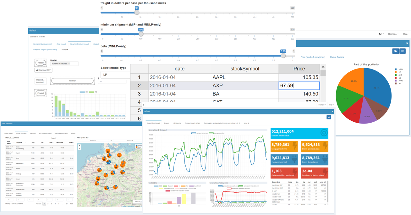
In this section you will learn how to customize GAMS MIRO. As you saw previously when creating your first app, MIRO launches without any further configuration. However, you will find that there are a lot of configuration possibilities to adapt MIRO to your specific model.
The configuration is done via a graphical configuration interface, with which you can create plots and widgets or change certain settings with a few mouse clicks, visually supported by a live preview. In addition, the configuration can also be done manually via a JSON file. In fact, all the graphical Configuration Mode does is create this JSON file.
The Configuration Mode is directly accessible via GAMS Studio:
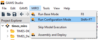
In order to launch the Configuration Mode via the command line, the environment variable MIRO_MODE=config needs to be set instead of MIRO_MODE=base. The other steps (see here) remain the same.
After starting, the following screen appears:
Changes made in the configuration are only effective after a restart of the MIRO application.
As the name suggests, general options can be set in this section (click on an item for more information).
MIRO allows you to run custom analysis scripts in both Base and Hypercube Mode. These scripts have to generate HTML output which will be displayed in the interface once the script finished. Scripts need to be placed in a folder called scripts_<modelname>; this is also where MIRO executes them (important when you use relative paths in your script).
All software needed to run the script must be installed on the client's machine and added to the PATH, as it is not part of a MIRO application.
In this section you can customize the general configuration of input and output tables (global settings) as well as the individual settings of multi-dimensional symbol tables.
By default, every cell in an input table is editable and rows can be inserted and removed. If you only want to allow your users to edit certain tables or even only certain columns within a table, you can customize the visualization for the underlying GAMS parameter. You can also use a different type of table to enter your data. For example, if you have large amounts of data (>100,000 records) in your table, we recommend using either the Big Data Table or the pivot table. In addition, input tables can be annotated with Markdown syntax. This way you can give your users additional information, e.g. what kind of data should be entered here and in which format.
Also global table settings for output symbols can be overwritten for each individual symbol. The available options are almost identical. The only additional settings are the number of decimal places to display and an option to disable graphics for the symbol.
Note that in contrast to the global settings, a symbol-specific configuration needs to be applied by clicking on the corresponding save-button!
Available options for an input symbol table (type: Default):
This is the standard table in MIRO, which works similar to a spreadsheet.
Available options for an input symbol table (type: Big Data Table):
This table type is intended for situations in which large amounts of data are to be displayed within a table. Instead of a long, 1-page table, a multi-page table is displayed. Only the data currently visible on the client side is loaded in this table.
Available options for an input symbol table (type: MIRO Pivot Table):
This table type is also capable of handling large amounts of data (> 1 million records). It allows you to interactively filter, pivot or aggregate data. See here for more information about the MIRO Pivot Table. The configuration of this table can be done directly from the preview on the right side.
The MIRO Pivot Table has no concept of "order" because the table can be sorted interactively by changing the order of the rows. When you add or change UELs, they are always appended to the underlying data source. So when MIRO passes the data to GAMS, you cannot rely on the order of the elements coming from this table type. If you need UELs in a certain order, you should either use one of the other input table types or declare the sets you need sorted as additional external input (instead of using the implicit set definition).
Available Options for an output symbol table:
For all other options please consult the section for global table settings.
Input widgets can be used instead of tables to enter scalar input data. Examples of such widgets include: sliders, dropdown menus, date selectors or checkboxes. In the configure widgets section of the Configuration Mode you can configure widgets for:
The section Configure widgets looks as follows:
The symbol type to be configured can be selected at the top. The options are:
After configuring a widget, the corresponding scalar is automatically removed from the Scalars table and rendered as a widget instead.
New GAMS option / New double dash parameter
As the name suggests, GAMS options and double-dash parameters can be configured here as an input widget.
Since those parameters are specified via the command line in GAMS, they can not be tagged in the GAMS code with $onExternalInput
/ $offExternalInput
. So that they can be set for a GAMS run via MIRO, they must be explicitly specified in the configuration.
If a GAMS option or a double dash parameter is set via MIRO, your GAMS model will automatically be called with these command line parameters. The values the user selected are therefore available to the GAMS model at compile time.
The GAMS options and double-dash parameters associated with a scenario are stored in MIRO's internal database. However, the information about them is lost when a scenario is exported as a GDX file. We therefore recommend using singleton sets instead of command line parameters. Both the element label and the element text of a set can be migrated to compile time variables using the Dollar Control Options eval.Set, evalGlobal.Set, and evalLocal.Set.
Read more here.
Example:
If we set the double dash parameter numberPeriods to 11 and for the GAMS option mip we select CPLEX from within MIRO, then the GAMS model is run with:
gams <modelname>.gms --numberPeriods=11 MIP=CPLEX
The following GAMS options are reserved by GAMS MIRO and can not be configured: idir1, idir2, curdir, trace, traceopt
The following widgets are available for scalar values:
Click on a widget to get more information
Example:
Let's now configure a widget for our transport model. For the scalar value freight a slider is a good choice.
From the list of available symbols we choose the desired scalar, select slider as widget tye and give it a label, which then appears above the slider.
Next, we specify the upper and lower bounds of the slider, the default value as well as the step size.
When we are satisfied with the selected configuration, we click "save". A confirmation that the configuration has been updated successfully will appear:
Done!
Besides the default tabular format, multidimensional GAMS symbols can be visualized as graphs. GAMS MIRO offers comprehensive visualization options. A lot of plotting types are available and only need to be configured, i.e. adapted to your model-specific data.
The following section shows some examples for different chart types you can use in MIRO. It is not useful to describe all possible options MIRO supports. Instead, you should just explore it yourself! Start the Configuration Mode and play around with the data until you get a satisfactory result.
To create graphics that are perfectly tailored to your data and not available in MIRO yet, you can also use MIRO's R-API. More information can be found here.
Create database backups, restore a database, remove database tables.
Deleting data from the database cannot be undone!
With the Configuration Mode we pursue the goal that a user can completely configure a MIRO application without having to write any JSON code. However, there are a few advanced options that are not yet available in the Configuration Mode and will have to be configured manually when desired. The following section describes these options.
The entire configuration of MIRO is done via JSON files. After the first start of a MIRO app, the following files are located in <modeldirectory>/conf_<modelname>:
$onExternalInput
/ $offExternalInput
and $onExternalOutput
/ $offExternalOutput
tags are listed here. You won't ever have to modify this file!
If you don't start MIRO via GAMS Studio but via the command line, the JSON files are not created automatically. Read more about this here.
In case you want to change the language of MIRO or display a scalar input symbol as a slider, this information must be stored in the <modelname>.json file in JSON syntax. When you first launch MIRO for a new model, the <modelname>.json file is almost empty:
{}
Each adjustment you want to make must be captured within the curly braces of this file.
To ensure that the configuration is correct in terms of syntax and content, all JSON files are validated against schema in the background.
Only if the validation is successful the application starts. If a schema is violated, an error message is displayed.
The schemas are located in <MIRORoot>/miro/conf. For the <modelname>_io.json this is the schema <MIRORoot>/miro/conf/io_config_schema.json and for the <modelname>.json the schema <MIRORoot>/miro/conf/config_schema.json is used.
Since the latter file is used for the configuration, only the corresponding schema is of interest. You can have a look at it here.
In the sections on configuring widgets and charts, you can also find examples of what the configuration looks like in JSON.
Let's get back and extend our demo model transport. We will do this by adjusting the file transport.json in order to to adapt MIRO to our needs.
GAMS MIRO comes with several options on how you can feed your model with input data. By default, GAMS input parameters, sets and scalars are displayed in an editable table:
The corresponding GAMS declaration statement looks like this: Parameter d(i,j) 'distance in thousands of miles';
.
By default, every cell in the table is editable and rows can be inserted and removed. If you only want to allow your users to edit certain tables or even only certain columns within a table, you can customize the visualization for the underlying GAMS parameter.
You do so by adding this kind of information to the transport.json file. For example, if we decide that the table for our parameter d should not be editable, this information needs to be added to our JSON file as follows:
{
"inputWidgets": {
"d": {
"widgetType": "table",
"readonly": true
}
}
}
As with all MIRO customizations, the information about the type of visualization of a GAMS scalar is configured via the file <modelname>.json.
Let's get back to our transport app. In the previous section we configured the table of parameter d so that it is no longer editable. We achieved this by writing the corresponding information into the transport.json file.
Now we extend the configuration of our app further by adding information about how to display the scalar value f ('freight in dollars per case per thousand miles'). Instead of displaying it in a table, we want to use a slider:
{
"inputWidgets": {
"d": {
"widgetType": "table",
"readonly": true
},
"f": {
"widgetType": "slider",
"alias": "Freight in dollars per case per thousand miles",
"label": "Select the freight costs",
"min": 1,
"max": 500,
"default": 90,
"step": 1
}
}
}
When we restart our app, the scalar is now automatically removed from the Scalars table and instead rendered as a separate widget:
In the sections on widgets and charts you will find a JSON example for each widget or chart type.
We have already mentioned the possibility of setting GAMS command line parameters via MIRO.
Since GAMS Options and Double Dash Parameters are specified via the command line in GAMS, they can not be tagged in the GAMS code with $onExternalInput
/ $offExternalInput
. To be able to set them from MIRO, they can be specified in the <modelname>.json file. In order for MIRO to recognize whether your symbol is a double dash parameter or a GAMS option, you must prefix the symbol name with either _gmspar_ for double dash parameters or _gmsopt_ for GAMS options.
Command line parameters can not be displayed as a table, but only as a widget. Both, GAMS options and double-dash parameters can be displayed as a slider, dropdown menu, checkbox, text input or numeric input. For double-dash parameters date(-range) selector and slider range are also available.
Let's assume you want MIRO to call your GAMS model with the double dash parameter --numberPeriods, which can be set to a value between 1 and 14. You also want to be able to select the MIP solver to use. As you have licenses for CPLEX, Gurobi and XPRESS, you can only use either of these three solvers. Thus, your <modelname>.json file could look as follows:
{
"inputWidgets": {
"_gmspar_numberPeriods": {
"widgetType": "slider",
"alias": "Number of time periods",
"label": "Select the number of time periods to solve",
"min": 1,
"max": 14,
"default": 11,
"step": 1
},
"_gmsopt_mip": {
"widgetType": "dropdown",
"alias": "MIP Solver",
"label": "Solver to use for MIP models",
"choices": [
"CPLEX",
"GUROBI",
"XPRESS"
],
"multiple": false,
"selected": "CPLEX"
}
}
}
The resulting interface in MIRO now looks as follows:
In the MIRO Base Mode, widgets with ranges are only available for double-dash parameters!
We covered the basics of how to use widgets for your scalar inputs as well as command line parameters. Let's now take a look at how widgets that return two scalars instead of one are treated. Those widgets include a slider with two handles (also referred to as a slider range) and a date range selector:
The lower value (or starting date of the date range) is postfixed with _lo and the upper value (or end date of the date range) is postfixed with _up. This means that if you specified a slider range for your double dash parameter --RANGE, you can access the lower value of the range with %RANGE$LO% and the upper value with %RANGE$UP% while %RANGE% will not be set at all. Let's look at the following example: We would like to specify a time window that we want to fetch stock data for. Thus, we define a new double dash parameter --TW that we want to be visualized in the form of a date range selector. We add the following JSON snippet to our <modelname>.json configuration file:
{
"inputWidgets": {
"_gmspar_TW": {
"alias": "time window",
"widgetType": "daterange",
"label": "Time window",
"start": "2018-02-20",
"end": "2019-02-20",
"min": "2017-01-01",
"max": "2019-12-31",
"autoclose": true,
"noHcube": true
},
[...]
In our model, we can access the lower and upper value of this slider via the compile time variables %TW$LO% and %TW$UP%.
One special feature of GAMS MIRO is that you can define interdependencies between different parameters. Scalars can take two forms of dependencies to other parameters: They can feed their attributes from them; and they can manipulate the content of those parameters. Let's look at an example: we have a set of scenarios that can be selected as well as a singleton set with the currently selected/active scenario. A singleton set is suited to be represented as a dropdown menu, hence we choose that type of widget here. We would like to filter our parameters based on the currently selected scenario so that we only see data that is relevant for this scenario (this type of dependency is also referred to as a backward dependency). This means that in case scenario 1 is selected via our dropdown menu, we only want to display data relevant to scenario 1 to the user. Additionally, we want the choices of our dropdown menu to be the elements of all available scenarios (also referred to as a forward dependency).
Similar dependencies can also be considered for sliders. An example is the pickstock model. Here, the number of stocks you can select for your portfolio can not be larger than the number of stocks in your dataset. Similarly, the number of days you can use to train your model must not be larger than the number of days you have in the stock price dataset. The slider attributes - namely the maximum value that can be selected - should change according to the price data the user uploads. Thus, we also have forward dependencies here.
A table that shows the currently supported forms of dependencies for the different input widgets is shown below.
Input widget type | Forward dependency | Backward dependency | Example model |
---|---|---|---|
Dropdown menu | - | ||
Slider | pickstock | ||
Checkbox | - | ||
Date selector | - | ||
Daterange selector | () | - |
You need dependency support for a type of widget which is currently not available? Please feel free to contact us at: miro@gams.com. You added dependency support for another type of widget yourself? Send us a pull request on GitHub!
GAMS MIRO allows you to use your own custom renderers for your datasets. In this section we will show you how to create really sophisticated graphics that can not be configured with the Configuration Mode of GAMS MIRO.
The following example shows how a map can be created using a custom renderer. Note that maps can also be configured in the Configuration Mode. However, the following example shows how the R API can be used for custom graphics in general.
In order to visualize a dataset, you will need to write two functions: a placeholder where your graphs etc. will later be rendered as well as the rendering function itself. To learn more about the concepts of this dual component approach, visit the website for the R Shiny framework that GAMS MIRO is based upon: https://shiny.rstudio.com/. In particular, we are using Shiny Modules to realize the interface between MIRO and your custom renderer functions. The template for the two components of every custom renderer is as follows:
<rendererName>Output <- function(id, height = NULL, options = NULL, path = NULL){
ns <- NS(id)
}
render<rendererName> <- function(input, output, session, data, options = NULL, path = NULL, views = NULL, ...){
}
Note that you need to replace <rendererName> with your preferred name. Let's go through this code step by step. As mentioned, for each custom renderer we need to specify two functions: one that generates the the placeholder and one that fills this placeholder with data. The name of the placeholder function must be postfixed with "Output" and the name of the function that specifies the actual rendering must be prefixed with the keyword "render". Let's get back to our transport example. We would like to see the flow of goods visualized on a map. We now write our own custom renderer which we name: transportMap. Thus, our initial template looks like this:
transportMapOutput <- function(id, height = NULL, options = NULL, path = NULL){
ns <- NS(id)
}
renderTransportMap <- function(input, output, session, data, options = NULL, path = NULL, views = NULL, ...){
}
R is case sensitive and the first letter after the render keyword needs to be uppercase! Thus, if the name of your renderer starts with a lowercase letter, you need to convert it to uppercase in the render* function.
Custom renderer scripts must be located in a folder named: renderer_<modelname> in your model directory. You can name these .r files as you like.
Both functions take a number of parameters. Let's start with the placeholder function: Each custom renderer has its own ID. In order to avoid name collisions with other custom renderers or functions of GAMS MIRO, we need to prefix our input and output elements with this ID. How should we prefix our custom input and output functions, though? Fortunately, Shiny provides us with the function: NS(). This function takes the ID of our custom renderer as its input and returns a function (functions that return functions are often called closures in R) that does the prefixing for us. Thus, whenever we want to specify a new input or output element, we simply hand the ID we would like to use for this element over to this prefixing function (which in our case is bound to the ns variable). We can also specify a height for our renderer as well as the path where the renderer files are located. We can also pass additional options to our renderer functions.
Let's get back to our example. As we would like to visualize our optimized schedule on an interactive map, we choose the popular Leaflet library. Fortunately, there is already an R/Shiny interface for this library: Leaflet for R. This R package comes with the two functions: leafletOutput() that generates the placeholder and renderLeaflet() that renders a Leaflet map object created by the leaflet() function which takes our dataframe as its first argument. So let's put the pieces together and extend our code:
transportMapOutput <- function(id, height = NULL, options = NULL, path = NULL){
ns <- NS(id)
leaflet::leafletOutput(ns("map"), height = height)
}
renderTransportMap <- function(input, output, session, data, options = NULL, path = NULL, views = NULL, outputScalarsFull = NULL, ...){
output$map <- leaflet::renderLeaflet(leaflet::leaflet(data))
}
Note that we used the aforementioned ns() function to prefix the ID ("map") that we chose for our Leaflet element. Just like any other placeholder element, the function leafletOutput() generates an element that can be accessed via the list-like output object.
Inside our rendering function we assign this object the Leaflet map that is created by the renderLeaflet() function. In case you find the whole concept of having an output function, a rendering function, an output object etc. still very confusing, you should take a look at the official tutorial series for the Shiny framework.
To summarize: elements that generate data can be accessed by the input object; elements that transform data to some form of visualization via the output object and any user-specific information via the session object.
If you use functions from packages other than shiny, DT, rhandsontable, dplyr, readr or the R base packages, make sure you specify the package/namespace that exports this function. In our example, the functions leafletOutput, renderLeaflet and leaflet are exported from the package leaflet. So we need to use the double colon operator to access them (e.g. leaflet::leafletOutput).
The data that you want to visualize is supplied to your rendering function by the data argument - an R tibble, a data structure that is very similar to a Data Frame. In case you specified additional datasets to be communicated with your custom renderer, data will be a named list of tibbles where the names are the GAMS symbol names. In addition, the values of all output scalars can be accessed via the argument outputScalarsFull (a tibble with the columns scalar, description, value). The function argument path is a string (a one-dimensional character vector) that specifies the absolute path to your renderer_<modelname> directory. This is useful if you want to include external files in your custom renderer functions. Optional parameters that you want to pass to the renderer can be accessed via the argument options - a (nested) list.
The list options always has a nested list with the key _metdata_, which gives you access to the metadata of the symbol to render, such as the symbol type (set, parameter, ...) and header information (header name, alias, type). For example, the symbol type can be accessed as follows: options[["_metadata_"]][["symtype"]]
.
Now that we are familiar with the template that every custom renderer builds upon, we are still missing one fundamental concept so that we can use our custom renderer: binding the renderer to dataset(s) we wish to visualize.
This binding of GAMS parameter to renderer function is specified - just like any other renderer binding - in the <modelname>.json file; more precisely the dataRendering section. Let's assume that in our transportation example the GAMS parameter that specifies the optimal schedule is defined as optSched(lngp, latp, lngm, latm, plant, market) where (lngP,latP) and (lngm, latm) are the coordinates of the plants and markets respectively. Our transport.json file should then look like this:
{
"dataRendering":{
"optSched":{
"outType":"transportMap",
"height":"700",
"options":{
"title":"Optimal transportation schedule"
}
}
}
}
As you can see we bound the GAMS parameter optSched to our new custom renderer transportMap. Furthermore, we specified a parameter: title that can be accessed by our custom renderer via the options list.
If we decided to run our MIRO app now, we still would not be able to see anything other than a blank area. Thus, we will need to fill our renderer with some life:
transportMapOutput <- function(id, height = NULL, options = NULL, path = NULL){
ns <- NS(id)
tagList(
textOutput(ns("title")),
leaflet::leafletOutput(ns("map"))
)
}
renderTransportMap <- function(input, output, session, data, options = NULL, path = NULL, views = NULL, ...){
output$title <- renderText(options$title)
output$map <- leaflet::renderLeaflet(leaflet::leaflet(data) %>%
leaflet::addTiles() %>%
leaflet::addMarkers(~lngp, ~latp, label = ~plant)
)
}
We have added a new placeholder for the title. Note the use of the tagList() function. Since every R function has a single return value which is either the last evaluated expression of the function or the argument to the first return() function that is encountered in the function body, we need to return a list object. A tagList() is simply a list with an additional attribute to identify that the elements are html tags.
Within our rendering function, we set the title, add the default OpenStreetMap tiles as well as some markers for our plants.
The syntax ~lngp that you see here is simply a shorthand for data$lngp - the pipe operator a(x) %>% b(y) a shorthand for tmp <- a(x); b(tmp, y)
You now know everything you need in order to get started writing your own custom renderers! Congratulations! In case you create a new renderer that you would like to share so that others can benefit from your work as well, please contact us!
A custom renderer for an output symbol can use the data of other GAMS symbols. For example - let's stay with the above example of a map - the geographical information can come from other symbols than the transport data. For a custom renderer to access this data, the corresponding symbols must be specified in the <modelname>.json file under "additionalData"
:
{
"dataRendering":{
"optSched":{
"outType":"transportMap",
"height":"700",
"options":{
"title":"Optimal transportation schedule"
},
"additionalData": ["symbol_a", "symbol_b"]
}
}
}
All symbols that a custom renderer should use must be included in the GAMS/MIRO data contract.
In a custom renderer you can include any R packages that are not part of MIRO. This allows you to use all data visualization and data processing capabilities of R. In order for such packages to be installed when starting a MIRO application, they must be specified in the <modelname>.json file at the configuration of the corresponding symbol under "packages"
:
{
"dataRendering":{
"optSched":{
"outType":"transportMap",
"height":"700",
"options":{
"title":"Optimal transportation schedule"
},
"additionalData": ["symbol_a", "symbol_b"],
"packages": ["package_a", "package_b"]
}
}
}
Note that these additional packages are installed but not loaded! This means that when you call the function, you must explicitly specify the package name using the Double Colon Operator: pkg::name(...). See also the info box in the previous section.
Additional R packages are installed in the workspace of GAMS MIRO the first time a MIRO application is started.
In cases where your renderers are interactive, you might want to allow users to store the current state of your renderer and load it later with a single click. This is what MIRO views were designed for. A MIRO view can be any (nested) list that is JSON serializable. Views are bound to a particular GAMS symbol and each view has a unique id. One example of a renderer where the MIRO views API is used is the pivot table renderer.
You might have already seen that there is another argument in the renderer function that we have not yet talked about: the views argument. This is a reference to an instance of the views R6 class. You can get, add and remove views as well as register callbacks via this object. The following section explains how to use the API.
views$get(session, id = NULL)
session | The session object passed to the custom renderer |
---|---|
id | id of the view to load |
In case id is NULL: a named list where the names are the ids of the views and the values are the view data.
In case id is not NULL: a list with the data of the view. Will throw an error in case the id provided does not exist.
This method allows you to retrieve the data of views registered for the symbol. You can retrieve either the data of all views (id is NULL) or the data of a specific view (id not NULL).
# myViews <- list(filter1 = list(filter = list(element1 = "Value 1", element2 = c("Value 2", "Value 4"))),
# filter2 = list(filter = list(element3 = "Value 7")))
views$get(session, "filter1")
#> $filter
#> $filter$element1
#> [1] "Value 1"
#>
#> $filter$element2
#> [1] "Value 2" "Value 4"
views$get(session)
#> $filter1
#> $filter1$filter
#> $filter1$filter$element1
#> [1] "Value 1"
#>
#> $filter1$filter$element2
#> [1] "Value 2" "Value 4"
#>
#>
#>
#> $filter2
#> $filter2$filter
#> $filter2$filter$element3
#> [1] "Value 7"
views$get(session, "filter3")
#> Error: View with id: filter3 could not be found.
views$getIds(session)
session | The session object passed to the custom renderer |
---|
Character vector with the view ids registered for the symbol.
Retrieves the view ids that are currently registered for the symbol. It is equivalent to names(views$get(session))
.
# myViews <- list(filter1 = list(filter = list(element1 = "Value 1", element2 = c("Value 2", "Value 4"))),
# filter2 = list(filter = list(element3 = "Value 7")))
views$getIds(session)
#> [1] "filter1" "filter2"
views$add(session, id, viewConf)
session | The session object passed to the custom renderer |
---|---|
id | id of the view to add |
viewConf | The view configuration |
Adds/registers a new view. The view configuration can be any JSON serializable list. If a view with the same id already exists for the symbol, the previous view is replaced. In case the current renderer is read-only (not a sandbox scenario), an error is thrown. You can test whether the renderer is read-only with the method views$isReadonly(session)
.
# myViews <- list(filter1 = list(filter = list(element1 = "Value 1", element2 = c("Value 2", "Value 4"))),
# filter2 = list(filter = list(element3 = "Value 7")))
views$add(session, "filter3", list(filter = list(element4 = "Value 10")))
views$remove(session, id)
session | The session object passed to the custom renderer |
---|---|
id | id of the view to remove |
Removes a view with the specified id. If no view with this id exists, an error is thrown. In case the current renderer is read-only (not a sandbox scenario), an error is thrown. You can test whether the renderer is read-only with the method views$isReadonly(session)
.
# myViews <- list(filter1 = list(filter = list(element1 = "Value 1", element2 = c("Value 2", "Value 4"))),
# filter2 = list(filter = list(element3 = "Value 7")))
views$get(session)
#> $filter1
#> $filter1$filter
#> $filter1$filter$element1
#> [1] "Value 1"
#>
#> $filter1$filter$element2
#> [1] "Value 2" "Value 4"
#>
#>
#>
#> $filter2
#> $filter2$filter
#> $filter2$filter$element3
#> [1] "Value 7"
views$remove(session, "filter2")
views$get(session, "filter1")
#> $filter
#> $filter$element1
#> [1] "Value 1"
#>
#> $filter$element2
#> [1] "Value 2" "Value 4"
views$remove(session, "filter2")
#> Error: View with id: filter2 does not exist, so it could not be removed.
views$registerUpdateCallback(session, callback)
session | The session object passed to the custom renderer |
---|---|
callback | a callback function |
You can register a callback function that is triggered whenever the view data of a symbol is modified outside the renderer. This happens when a user modifies the view data via the metadata dialog. Note that the callback function is not triggered by the methods views$add
or views$remove
described above.
updateCallback <- function(){
print(sprintf("View data changed from outside! New view ids: %s.",
views$getIds(session)))
}
views$registerUpdateCallback(session, updateCallback)
GAMS MIRO comes with the ability to change the preferred language. Setting your preferred language results in MIRO embedding the corresponding language file where all the language specific components are specified via JSON syntax. MIRO currently ships with three of those language files: English, German and Chinese. If you would like to add another language to this list, you are more than welcome to translate one of the existing language files. The language files are located at: <MIRORoot>/miro/conf/en.json and are validated against the JSON Schema file: <MIRORoot>/miro/conf/language_schema.json. Note that there are sometimes placeholders in the language files. Let's take the error message: "The value '%s' for the slider: '%s' is not of numeric type." for example. %s will then be replaced with the value and name of the slider by MIRO. Thus, if you create a new language file, be sure to include these placeholders there!
If you would like to contribute your language file, so that other people can profit from your work as well, send us an email: miro@gams.com.