Options not Available in Configuration Mode

    Custom data connectors

    MIRO allows you to import and export scenario data in a number of file formats. However, you may have data in a custom format that MIRO does not support, or you may want to pull and push data directly from an external database. In these cases, you need to write your own data connector in the form of an R function that you can connect to MIRO. Custom data connectors should be saved as miroimport.R or miroexport.R files and placed in the renderer_<modelname> directory.

    MIRO allows you to define multiple import and multiple export functions. They are accessible via the Load data and Export scenario dialogs.

    Custom data import and export functions displayed in the data load and export dialogs
    Custom import functions

    The custom import function should have the following signature:

    
    miroimport_<importerName> <- function(symNames, localFile = NULL, views = NULL, attachments = NULL, metadata = NULL, customRendererDir = NULL, ...) {
    
    }

    where importerName can be any name of your choice to identify the importer, symNames is a character vector with the names of the symbols to fetch data for and localFile is an optional data frame with one row for each uploaded file and the columns: name that specifies the name of the uploaded file, size that specifies the file size in bytes, type that provides the MIME type reported by the browser and datapath with the temporary path where the file was uploaded to. In addition, you have access to the metadata, attachments and views of the sandbox scenario. The directory renderer_<modelname> can be accessed via the customRendererDir argument (e.g. to access additional files placed in the same directory).

    The custom import function should return a named list of data frames or tibbles, where the names are the symbol names. Any errors thrown by your custom import function will be caught by MIRO and a generic error message will be displayed to the user. If you want to give the user a more informative error message, you can trigger a custom error with the abortSafe(msg = "") function. The msg will be displayed to the user.

    Let's create a custom import function for our transport example that allows us to upload data in the form of JSON files. We will use the jsonlite package to parse the JSON data. First, we create a file miroimport.R in the renderer_transport directory. Second, we write our own import function:

    miroimport_JSON <- function(symbolNames, localFile = NULL, views = NULL, attachments = NULL, metadata = NULL, customRendererDir = NULL, ...) {
      if (is.null(localFile) || !identical(length(localFile$datapath), 1L)) {
        abortSafe("Please upload a single, valid JSON file")
      }
      tryCatch(
        {
          jsonData <- jsonlite::read_json(localFile$datapath, simplifyVector = TRUE)
        },
        error = function(e) {
          abortSafe("Could not parse JSON file. Is the syntax correct?")
        }
      )
      dataTmp <- lapply(symbolNames, function(symbolName) {
        if (!symbolName %in% names(jsonData)) {
          return(NULL)
        }
        tryCatch(
          {
            return(tibble::as_tibble(jsonData[[symbolName]]))
          },
          error = function(e) {
            abortSafe("Could not parse JSON file. It does not seem to follow the expected structure.")
          }
        )
      })
      names(dataTmp) <- symbolNames
      return(dataTmp)
    }

    To use our newly created custom import function, we need to add the following configuration to our transport.json file:

    {
      "customDataImport": [
        {
          "label": "JSON import",
          "functionName": "miroimport_JSON",
          "symNames": ["a", "b"],
          "localFileInput": {
            "label": "Please upload your JSON file here",
            "multiple": false,
            "accept": [".json", "application/json"]
          }
        }
      ]
    }

    The label is used in the Data Import section as the identifier for our custom importer. functionName must be set to the name of the import function, in our case: miroimport_JSON.

    Also, we can use the symNames setting to restrict which symbols our import function supports. If we omit this setting, MIRO assumes that our import function supports any input and output symbol.

    The optional localFileInput object tells MIRO that our custom import function expects a local file to be uploaded. If the importer does not need a file (e.g. if it only fetches current values from a remote database), we can omit this object.

    To learn more about the different configuration options for custom import functions, below is the full schema against which your configuration will be validated.

    JSON validation schema for custom import functions
    "customDataImport": {
      "description": "Import data using a custom function",
      "type": "array",
      "items": {
        "type": "object",
        "additionalProperties": false,
        "required": [
          "label",
          "functionName"
        ],
        "properties": {
          "label": {
            "description": "Label that is displayed when selecting the custom importer",
            "type": "string",
            "minLength": 1
          },
          "symNames": {
            "description": "Names of the symbols to import. Defaults to all symbols (input and output) if not provided or empty.",
            "type": [
              "array",
              "string"
            ],
            "minLength": 1,
            "uniqueItems": true,
            "items": {
              "type": "string",
              "minLength": 1
            }
          },
          "functionName": {
            "description": "Name of custom R function to call (required function signature: miroimport(symNames, localFile = NULL, ...), must return named list of data frames with correct number/type of columns). The names of the list must be identical to the names provided by symNames argument.",
            "type": "string",
            "default": "miroimport",
            "minLength": 1
          },
          "localFileInput": {
            "description": "Enable user to provide local file.",
            "type": "object",
            "additionalProperties": false,
            "required": [
              "label"
            ],
            "properties": {
              "label": {
                "description": "Label of the local file input.",
                "type": "string"
              },
              "multiple": {
                "description": "Whether user is allowed to upload multiple files.",
                "type": "boolean"
              },
              "accept": {
                "description": "A character vector of unique file type specifiers which gives the browser a hint as to the type of file the server expects. Many browsers use this to prevent the user from selecting an invalid file.",
                "type": "array",
                "items": {
                  "type": "string"
                }
              }
            }
          }
        }
      }
    }
    Custom export functions

    For exporting data, a custom export function with the following signature should be used:

    
    miroexport_<exporterName> <- function(data, path = NULL, views = NULL, attachments = NULL, metadata = NULL, customRendererDir = NULL, ...) {
    
    }

    where data is a named list of tibbles, where the names are the names of the symbols (the same structure as the return value of a custom import function), and path is the file path of the (temporary) file provided to the user for download (optional). In addition, you have access to the metadata, attachments and views of the sandbox scenario. The directory renderer_<modelname> can be accessed via the customRendererDir argument (e.g. to access additional files placed in the same directory).

    Let's write a JSON export function that creates JSON files that can be re-imported using the custom import function from earlier. To do so, we first create a file miroexport.R in the renderer_transport directory. Then we write the custom export function:

    miroexport_JSON <- function(data, path = NULL, views = NULL, attachments = NULL, metadata = NULL, customRendererDir = NULL, ...) {
      jsonlite::write_json(data, path = path, dataframe = "columns")
    }

    and add the following to the transport.json file:

    {
      "customDataExport": [
        {
          "label": "JSON export",
          "functionName": "miroexport_JSON",
          "localFileOutput": {
            "filename": "output.json",
            "contentType": "application/json"
          }
        }
      ]
    }

    You will notice that the configuration object is very similar to that of the custom import functions, except that the optional localFileOutput object now specifies the properties of the file to be downloaded. We can omit this object if our export function does not create a file to be downloaded, but forwards the data to a remote service, for example.

    Below is the validation schema for custom exporters:

    JSON validation schema for custom export functions
    "customDataExport": {
      "description": "Export data using a custom function",
      "type": "array",
      "items": {
        "type": "object",
        "additionalProperties": false,
        "required": [
          "label",
          "functionName"
        ],
        "properties": {
          "label": {
            "description": "Label that is displayed when selecting the custom exporter",
            "type": "string",
            "minLength": 1
          },
          "symNames": {
            "description": "Names of the symbols to export. Defaults to all symbols (input and output) if not provided or empty.",
            "type": [
              "array",
              "string"
            ],
            "minLength": 1,
            "uniqueItems": true,
            "items": {
              "type": "string",
              "minLength": 1
            }
          },
          "functionName": {
            "description": "Name of custom R function to call (required function signature: miroexport(data, ...) where data is a named list of data frames, where the names are the names of the symbols).",
            "type": "string",
            "default": "miroexport",
            "minLength": 1
          },
          "localFileOutput": {
            "description": "Enable user to download file.",
            "type": "object",
            "additionalProperties": false,
            "required": [
              "filename"
            ],
            "properties": {
              "filename": {
                "description": "Name of the file (including extension) that users web browser should default to.",
                "type": "string",
                "minLength": 1
              },
              "contentType": {
                "description": "MIME type of the file to download. Defaults to application/octet-stream if file extension is unknown.",
                "type": "string",
                "minLength": 1
              }
            }
          }
        }
      }
    }
    Note:

    If you need to use credentials in your custom import/export functions (for example, to connect to a remote database service), you can provide them using environment variables (MIRO Desktop / MIRO Server).

    DEPRECATED: Remote data import and export

    Warning:

    This function is deprecated as of MIRO 2.3 and should no longer be used. It will be removed in one of the next MIRO versions! Please use the custom data connectors instead.

    A MIRO application can be supplied with data from various sources:

    • Internal database: Import existing scenario data
    • Local files: GDX, Excel
    • Manually entered data

    In addition to these default interfaces, the data can also come from or go to external sources.

    This MIRO data connector is implemented as a REST service. To set up a new external data source, you have to edit the <modelname>.json file which is located in the directory: conf_<modelname>. The following example shows how to set up an external data source to populate the symbol price:

    "remoteImport": [
        {
        "name": "Importer",
          "templates": [
            {
              "symNames": "price",
              "url": "http://127.0.0.1:5000/io",
              "method": "GET",
              "authentication": {
                "username": "@env:API_USER",
                "password": "@env:API_PASS"
              },
              "httpBody": [
                {
                  "key": "filename",
                  "value": "/Users/miro/Documents/importer/pickstock/price_data.csv"
                }
              ]
            }
          ]
        }
      ]

    The configuration of external data sources is template-based. This means that you can specify one and the same template for multiple input symbols. First, we have to specify which input symbols this template should apply to. Then we have to tell MIRO about the endpoint to connect to (in this case a server running on localhost on port 5000). Supported protocols are HTTP and HTTPS.

    When the user requests to import data via this data source "Importer", the resulting HTTP request looks as follows: GET /io?filename=%2FUsers%2Fmiro%2FDocuments%2Fimporter%2Fpickstock%2Fprice_data.csv&modelname=pickstock&dataset=price HTTP/1.1. When observing the request, you will notice that in addition to the filename key that you specified, MIRO sends two more key-value pairs: modelname and dataset set to the name of the model and dataset being requested. These will always be appended to the body provided by you.

    MIRO waits for the REST endpoint to respond with the requested dataset. Before we talk about the format in which MIRO expects the data, let's look at how the data is exported from MIRO to a remote destination. The format MIRO exports data is the same as data should be sent to MIRO!

    One more aspect worth talking about is authentication. When your API is not running on the local machine, but a remote server, you might want to provide credentials with your request. In the example above, we provided the username and password used to authenticate to the API. However, instead of hardcoding these credentials in the configuration file (which is possible), it is recommended to use the special prefix @env: that instructs MIRO to read the credentials from environment variables. Currently, the only supported authentication method is basic access authentication. In case you need another method, send us an email or a pull request!

    Warning:

    When using basic access authentication, username and password are sent in plain text! Therefore, you have to use HTTPS instead of HTTP to provide confidentiality!!

    Instead of importing data from a remote data source, you can also export data to a remote destination. In this example the data of the symbol stock_weight should be exported to a CSV file: export_stock_weight.csv. As we now push data to the API, we use the POST HTTP method. The structure of the JSON configuration is identical to that of remote importers you have seen before:

    "remoteExport": [
        {
          "name": "Exporter",
          "templates": [
            {
              "symNames": "stock_weight",
              "url": "http://127.0.0.1:5000/io",
              "method": "POST",
              "authentication": {
                "username": "@env:API_USER",
                "password": "@env:API_PASS"
              },
              "httpBody": [
                {
                  "key": "filename",
                  "value": "/Users/miro/Documents/exporter/pickstock/export_stock_weight.csv"
                }
              ]
            }
          ]
        }
      ]

    What's more interesting is the request body that MIRO sends to the remote server:

    {"data":[{"symbol":"AXP","value":0.472295069483016},{"symbol":"MMM","value":0.316292266161662},{"symbol":"MSFT","value":0.406195141778428}],"modelname":"pickstock","dataset":"stock_weight","options":{"filename":"/Users/miro/Documents/importer/pickstock/price_data.csv"}}

    MIRO sends data serialized as JSON. The modelname and dataset keys are sent along just like in the GET request we saw previously when importing data. In addition, we get the custom key-value pairs we specified in a special object called options as well as the actual data of the symbol in data. Note how the table is serialized. In case you need MIRO to serialize tables in a different format, send us an email or a pull request.

    Custom input widgets

    MIRO has an API that allows you to use custom input widgets such as charts to produce input data. This means that input data to your GAMS model can be generated by interactively modifying a chart, a table or any other type of renderer.

    Before reading this section, you should first study the chapter about custom renderers. Custom widgets are an extension of custom renderers that allow you to return data back to MIRO.

    Note:

    The API of the custom input widgets has been changed with MIRO 2.0. Documentation for API version 1 (MIRO 1.x) can be found in the MIRO GitHub repository.

    To understand how this works, we will look at an example app that allows you to solve Sudokus. We would like to visualize the Sudoku in a 9x9 grid that is divided into 9 subgrids - 3x3 cells each. We will use the same tool that we use to display input tables in MIRO, but we could have used any other R package or even a combination of those. Let's first look at the boilerplate code required for any custom input widget:

    
    mirowidget_<symbolName>Output <- function(id, height = NULL, options = NULL, path = NULL){
      ns <- NS(id)
    }
    
    renderMirowidget_<symbolName> <- function(input, output, session, data, options = NULL, path = NULL, rendererEnv = NULL, views = NULL, ...){
      return(reactive(data()))
    }
                                          

    You will notice that the boilerplate code for custom widgets is almost identical to that of custom renderers. The main difference to a custom renderer is that we now have to return the input data to be passed to GAMS. Note that we return the data wrapped inside a reactive expression. This will ensure that you always return the current state of your data. When the user interacts with your widget, the data is updated.

    The other important difference from custom renderers is that the data argument here is also a reactive expression (or a list of reactive expressions in case you specified additional datasets to be communicated with your widget), NOT a tibble.

    Let's get back to the Sudoku example we mentioned earlier. We place a file mirowidget_initial_state.R within the custom renderer directory of our app: <modeldirectory>renderer_sudoku. The output and render functions for custom widgets should be named mirorwidget_<symbolName>output and renderMirowidget_<symbolName> respectively, where symbolName is the lowercase name of the GAMS symbol for which the widget is defined.

    To tell MIRO about which input symbol(s) should use our new custom widget, we have to edit the sudoku.json file located in the <modeldirectory>/conf_<modelname> directory. To use our custom widget for an input symbol named initial_state in our model, the following needs to be added to the configuration file:

    {
    "inputWidgets": {
        "initial_state": {
          "widgetType": "custom",
          "rendererName": "mirowidget_initial_state",
          "alias": "Initial state",
          "apiVersion": 2,
          "options": {
            "isInput": true
          }
        }
      }
    }

    We specified that we want an input widget of type custom for our GAMS symbol initial_state. Furthermore, we declared an alias for this symbol which defines the tab title. We also provided a list of options to our renderer functions. In our Sudoku example, we want to use the same renderer for both input data and output data. Thus, when using our new renderer for the input symbol initial_state, we pass an option isInput with the value true to our renderer function.

    Note:

    For backward compatibility reasons, you currently need to explicitly specify that you want to use API version 2 for custom input widgets. In a future version of MIRO, this will become the default.

    Let's concentrate again on the renderer functions and extend the boilerplate code from before:

    
    mirowidget_initial_stateOutput <- function(id, height = NULL, options = NULL, path = NULL){
      ns <- NS(id)
      rHandsontableOutput(ns('sudoku'))
    }
    
    renderMirowidget_initial_state <- function(input, output, session, data, options = NULL, path = NULL, rendererEnv = NULL, views = NULL, ...){
      output$sudoku <- renderRHandsontable(
        rhandsontable(if(isTRUE(options$isInput)) data() else data,
                      readOnly = !isTRUE(options$isInput),
                      rowHeaders = FALSE))
      if(isTRUE(options$isInput)){
        return(reactive(hot_to_r(input$sudoku)))
      }
    }
                                          

    Let's disect what we just did: First, we defined our two renderer functions mirowidget_initial_stateOutput and renderMirowidget_initial_state. Since we want to use the R package rhandsontable to display our Sudoku grid, we have to use the placeholder function rHandsontableOutput as well as the corresponding renderer function renderRHandsontable. If you are wondering what the hell placeholder and renderer functions are, read the section on custom renderers.

    Note that we use the option isInput we specified previously to determine whether our table should be read-only or not. Furthermore, we only return a reactive expression when we use the renderer function to return data - in the case of a custom input widget. Note that for input widgets, we need to run the reactive expression (data()) to get the tibble with our input data. Whenever the data changes (for example, because the user uploaded a new CSV file), the reactive expression is updated, which in turn causes our table to be re-rendered with the new data (due to the reactive nature of the renderRHandsontable function). The concept of reactive programming is a bit difficult to understand at first, but once you do, you'll appreciate how handy it is.

    A detail you might stumble upon is the expression hot_to_r(input$sudoku). This is simply a way to deserialize the data coming from the UI that the rhandsontable tool provides. What's important is that we return an R data frame that has exactly the number of columns MIRO expects our input symbol to have (in this example initial_state).

    That's all there is to it! We configured our first custom widget. To use the same renderer for the results that are stored in a GAMS symbol called result, simply add the following lines to the sudoku.json file. Note that we do not set the option isInput here.

    "dataRendering": {
        "results": {
          "outType": "mirowidget_initial_state"
        }
      }

    The full version of the custom widget described here as well as the corresponding GAMS model Sudoku can be found in the MIRO model library. There you will also find an example of how to create a widget that defines multiple symbols. In this case, the data argument is a named list of reactive expressions, where the names are the lowercase names of the GAMS symbols. Similarly, you must also return a named list of reactive expressions. Defining a custom input widget for multiple GAMS symbols is as simple as listing all the additional symbols you want your widget to define in the "widgetSymbols" array of your widget configuration. Below you find the configuration for the initial_state widget as used in the Sudoku example.

    "initial_state": {
      "widgetType": "custom",
      "rendererName": "mirowidget_initial_state",
      "alias": "Initial state",
      "apiVersion": 2,
      "widgetSymbols": ["force_unique_sol"],
      "options": {
        "isInput": true
      }
    }

    In addition to defining a widget for multiple symbols, MIRO also allows you to access values from (other) input widgets from your code. To do this, you must list the symbols you want to access in the "additionalData" array of your configuration.

    Note that custom widgets cannot be automatically expanded to use them for Hypercube jobs. Therefore, if you include scalar symbols in custom widgets (either as the symbol for which the widget is defined or via "widgetSymbols") and still want to include these symbols in the Hypercube job configuration, you must also define a scalar widget configuration for Hypercube jobs. You can do this with the "hcubeWidgets" configuration option. Below you will find an example of the scalar force_unique_sol, which is to be used both as a custom widget and as a slider in the Hypercube module:

    {
      "activateModules": {
        "hcubeModule": true
      },
      "hcubeWidgets": {
        "force_unique_sol": {
          "widgetType": "checkbox",
          "alias": "Force initial solution",
          "value": 1,
          "class": "checkbox-material"
        }
      },
      "inputWidgets": {
        "force_unique_sol": {
          "widgetType": "custom",
          "rendererName": "mirowidget_force_unique_sol",
          "alias": "Initial state",
          "apiVersion": 2,
          "widgetSymbols": ["initial_state"],
          "options": {
            "isInput": true
          }
        }
      }
    }

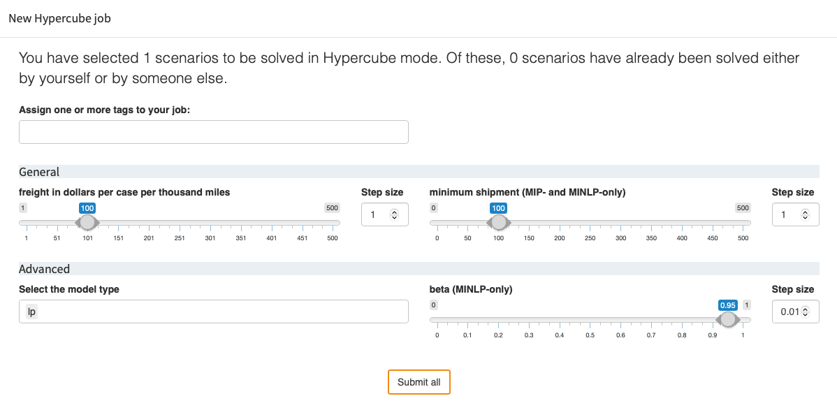
    The checkbox is then expanded to a dropdown menu in the Hypercube submission dialog (see this table, which widgets are supported and how they are expanded in the Hypercube submission dialog).

    Drop-down menu in input table

    An input table can be configured so that the cells are not freely editable by the user, but can only be modified via a drop-down menu. This can greatly simplify the usability of input tables. When used properly, another advantage of providing dropdown menus is the prevention of invalid or inconsistent user input data.

    The configuration of the drop-down menus is done column by column. In the following figure the column 'canning plants' (GAMS symbol Table d(i,j) 'distance in thousands of miles') has been configured to use a drop-down menu:

    Dropdown menu instead of normal cell

    The choices of a drop-down menu can be either predefined (static choices) or filled dynamically:

    • Static choices:
      Static choices are predefined in the <modelname>.json file by the app developer. The following configuration results in the drop-down menu in the figure above:
      {
        "inputWidgets": {
          "d": {
            "widgetType": "table",
            "alias": "distance in thousands of miles",
      	  "pivotCols": "j",
      	  "dropdownCols": {
              "i": {
                "static": ["Seattle", "San-Diego", "Los Angeles", "Houston", "Philadelphia"],
      		  "colType": "dropdown"
              }
            }
          }
      }

      The configuration is done in section "inputWidgets" for each input table (here: d) separately. In "dropdownCols" the individual table columns are specified (here: column "i"), which should have drop-down menus. The key "static" followed by an array defines the static drop-down choices. For the "colType" key you can choose between "dropdown" and "autocomplete" (default). While "dropdown" always displays all choices at once, "autocomplete" updates the displayed choices according to an autocomplete.

      Tip:

      If your configuration file does not yet have any entries for the table to be configured, you can simply create an initial configuration using the Configuration Mode. Select the desired symbol under "Tables" → "Symbol tables" and click on save. Make sure that "default" is selected as table type to be used.

      Table configuration
    • Dynamic choices:

      Choices are dynamically filled by the cells of a column in another table. In the following example, the GAMS symbol Table d(i,j) 'distance in thousands of miles' is configured so that the column i ("canning plants") displays a drop-down menu whose choices are fetched from the entries in the column of the same name in the symbol table a ("Capacity").

      This is what happens in the app: In the table "Capacity" the user can make any entries. If she edits the column "canning plants", the entries there are passed as choices to the dropdown menu of the "distance in thousands of miles" table:

      Dynamic dropdown choices

      The configuration of this table looks as follows:

      {
        "inputWidgets": {
          "d": {
            "widgetType": "table",
            "alias": "distance in thousands of miles",
      	  "pivotCols": "j",
      	  "dropdownCols": {
              "i": {
                "symbol": "a",
                "column": "i",
      		  "colType": "dropdown"
              }
            }
          }
      }

      Instead of a "static" key, there are now two keys "symbol" and "column". The value of the "symbol" key ("a" → "capacity" table) defines the symbol table whose "column" ("i" → "canning plants") is to be used to fill the drop-down menu.

    "dropdownCols":{
      "description":"Columns where only certain values are allowed to be selected (only supported for default tables)",
      "type":"object",
       "additionalProperties":{
          "type":"object",
          "properties":{
            "colType":{
              "description": "Column type (default is 'autocomplete')",
              "type":"string",
              "enum":["autocomplete", "dropdown"]
            },
            "static":{
              "description": "Arrays of static choices allowed for this column",
              "type":["array", "string"],
              "minLength":1,
              "items":{
                "type":"string",
                "minLength":1
              }
            },
            "symbol":{
              "description": "Symbol to fetch choices from",
              "type":"string",
              "minLength":1
            },
            "column":{
              "description": "Column (of symbol) to fetch choices from",
              "type":"string",
              "minLength":1
            }
          }
       }
    }
    Note:
    • The drop-down menu feature is only supported for the default input table type, not for big data tables or pivot tables.
    • User data is validated only during manual edits, i.e. when the user directly edits the values of individual cells. When the data is imported from external files or the database, there is no validation between the data and the drop-down menu choices.
    • If you have edited the table configuration of a symbol manually in the <modelname>.json file, you should not use the Configuration mode for this symbol anymore. This could overwrite your manual edits!

    Column validation in input table

    In addition to using dropdown menus, numeric columns of an input table can be configured to validate manual edits by the user against predefined criteria. As with dropdown menu columns, the configuration is done column by column. The following criteria are available:

    • min: Minimum value to accept
    • max: Maximum value to accept
    • choices: A vector of acceptable numeric choices. It will be evaluated after min and max if specified.
    • exclude: A vector of unacceptable numeric values
    • allowInvalid: Logical specifying whether invalid data will be accepted. Invalid data cells will then be colored red.

    The configuration is done in section inputWidgets for each input table separately. In validateCols the individual table columns are specified, which should be validated. In the following example a symbol d is used. Column 'new-york' has been configured so that only values between 1-10 are considered valid, excluding 9. If the user enters a non-valid value, MIRO accepts it, but highlights the corresponding cell in red. In the column 'topeka' only the values 11, 12 and 14 are accepted.

      "inputWidgets": {
        "d": {
          "widgetType": "table",
          "tableType": "default",
          "readonly": false,
          "hideIndexCol": false,
          "heatmap": false,
          "validateCols": {
            "new-york": {
              "min": 1,
              "max": 10,
              "exclude": 9,
              "allowInvalid": true
            },
            "topeka": {
              "choices": [11, 12, 14],
              "allowInvalid": false
            }
          }
        }
      }
    Tip:

    If your configuration file does not yet have any entries for the table to be configured, you can simply create an initial configuration using the Configuration Mode. Select the desired symbol under "Tables" → "Symbol tables" and click on save. Make sure that "default" is selected as table type to be used.

    Table configuration
    "validateCols":{
      "description":"Column values are validated against custom user criteria (only supported for default tables)",
      "type":"object",
       "additionalProperties":{
          "type":"object",
          "properties":{
            "min":{
              "description": "Minimum value allowed for this column",
              "type":["number"]
            },
            "max":{
              "description": "Maximum value allowed for this column",
              "type":["number"]
            },
            "choices":{
              "description": "Array of acceptable numeric values for this column",
              "type":["array", "number"],
              "minLength":1,
              "items":{
                "type":"number",
                "minLength":1
              }
            },
            "exclude":{
              "description": "Array of unacceptable numeric values for this column",
              "type":["array", "number"],
              "minLength":1,
              "items":{
                "type":"number",
                "minLength":1
              }
            },
            "allowInvalid":{
             "description":"Boolean that specifies whether invalid data will be accepted. Invalid data cells will be colored red.",
             "type":"boolean"
            }
          }
       }
    }
    Note:
    • The column validation feature is only supported for the default input table type, not for big data tables or pivot tables.
    • User data is validated only during manual edits, i.e. when the user directly edits the values of individual cells. Data imported from external files or the database is not validated.
    • If you have edited the table configuration of a symbol manually in the <modelname>.json file, you should not use the Configuration Mode for this symbol anymore. This could overwrite your manual edits!

    Column width of an input table

    With the colWidths option it is possible to adjust the column width of individual tables (in pixels). The Configuration Mode supports the specification of one column width for all columns of the table. To specify the width of each column individually, the <modelname>.json file must be modified manually. Note that using individual column widths is not compatible with the pivotCols option.

    Example:

    {
      "inputWidgets": {
        "d": {
          "widgetType": "table",
          "tableType": "default",
          "readonly": false,
          "hideIndexCol": false,
          "heatmap": false,
          "colWidths": [165, 200, 50]
        }
    }

    Default Views in Pivot Compare Mode

    Just as you can configure an external default view for an input/output symbol with a MIRO Pivot renderer, you can also select a default view for the same symbol in Pivot compare mode. The external view can be either a local (scenario-specific) or a global (app-wide) view.

    Note that the symbol name has to be prefixed with _pivotcomp_ to indicate that it is a pivot comparison mode view configuration. Also note that the symbol has an additional dimension with the special name _scenName, where the information about the scenario name is stored.

    Below is an example configuration for the output symbol schedule of the transport example:

    {
      "_pivotcomp_schedule": {
        "test" {
          "rows": ["i", "j"],
          "cols": {
            "_scenName": null
          },
          "filter": {
            "Hdr": "quantities"
          },
          "pivotRenderer": "bar"
        }
      }
    }
    To make this the default view, store the view configuration either as a scenario-specific local view or as a global view in the conf_transport/views.json file. Then, simply add the following configuration to your conf_transport/transport.json configuration file:
    {
      "pivotCompSettings": {
        "symbolConfig": {
          "schedule": {
            "externalDefaultView": "test"
          }
        }
      }
    }

    Custom scenario comparison

    GAMS MIRO natively supports three modes for scenario comparison: split view, tab view, and pivot view. But what if you are interested in different statistics or charts tailored to compare multiple scenarios? For this purpose, there are user-defined scenario comparison modules. The data can be loaded into the custom comparison modules via the Batch Load module. The drop-down menu for selecting the comparison mode in which the selected scenarios are to be loaded is expanded accordingly.

    Custom comparison module selection in Batch Load module

    Custom scenario comparison modules work in a similar way to custom renderers. Therefore, we strongly recommend that you read the chapter on custom renderers first. Just like a custom renderer, a custom scenario comparison module consists of a JSON configuration block and an .R file containing the code in your application's renderer directory (renderer_<modelname>). Let's go through this process by creating a new comparison module for the pickstock model.

    We start by creating the boilerplate code for our renderer in a new file mirocompare_<id>.R inside the renderer_pickstock directory where <id> is the ID of our custom comparison module. The ID can be freely chosen. It must be 2-20 characters long and contain only ASCII lowercase letters or digits. We choose the name maxstock1 for our example and create the file mirocompare_maxstock1.R accordingly.

    Just like custom renderers, custom scenario comparison modules consist of two functions: the placeholder or output function and the renderer function:

    
    mirocompare_<id>Output <- function(id, height = NULL, options = NULL, path = NULL) {
      ns <- NS(id)
    }
    
    renderMirocompare_<id> <- function(input, output, session, data, options = NULL, path = NULL, rendererEnv = NULL, views = NULL, ...) {
    }

    If you have already written your own renderers, the argument list of the output and renderer functions will look familiar. Therefore, we will focus on the differences: First, unlike custom renderers, the data argument is not a dataframe, but an R6 object of class CustomComparisonData. The different methods of this class are described in the next section. Second, you have access to the attachment data of the scenarios via the data$getAttachmentData() method instead of a separate object.

    Views can be used in custom comparison renderers just like in custom renderers for output data.

    Let's return to our example and write an initial renderer that plots the relative test error against the maximum number of stocks.

    
    mirocompare_maxstock1Output <- function(id, height = NULL, options = NULL, path = NULL) {
      ns <- NS(id)
      return(plotOutput(ns("maxstockVsErrorTest")))
    }
    
    renderMirocompare_maxstock1 <- function(input, output, session, data, options = NULL, path = NULL, rendererEnv = NULL, views = NULL, ...) {
      scalarsPivoted <- dplyr::bind_rows(lapply(data$get("_scalars"), tidyr::pivot_wider, names_from = "scalar", values_from = "value", id_cols = character()))
      scalarsOutPivoted <- dplyr::bind_rows(lapply(data$get("_scalars_out"), tidyr::pivot_wider, names_from = "scalar", values_from = "value", id_cols = character()))
      scalars <- suppressWarnings(dplyr::mutate(dplyr::bind_cols(scalarsPivoted, scalarsOutPivoted), across(everything(), as.numeric)))
      scalars[["error_test_rel"]] <- scalars[["error_test"]] / scalars[["trainingdays"]]
    
      output$maxstockVsErrorTest <- renderPlot(boxplot(error_test_rel ~ maxstock, scalars, main = options$chartTitle))
    }

    We first use the get() method of the data object to retrieve input and output scalars. Scalars are treated specially in that they are bundled into a single data frame with the columns: scalar, description and value. Therefore, we must first pivot them and merge the input and output scalars. Then we can calculate a new derived column error_test_rel and create a boxplot with this relative test error against the maximum number of stocks.

    In order to use this custom comparison module in MIRO, we have to append the following JSON configuration to the pickstock.json file in the conf_pickstock directory:

    {
      "customCompareModules": [
        {
          "id": "maxstock1",
          "label": "Test error against maximum stocks",
          "options": {
            "chartTitle": "Testing error (rel.) vs maximum number of stocks"
          }
        }
      ]
    }

    The only mandatory fields are id and label. The label is displayed when selecting the comparison mode and the id is used internally to identify your module. You can specify an optional object with options provided to the output and renderer functions. This is especially useful if you want to reuse the same renderer function with different options. In this case, the id of the comparison module is not the same as the id of the output/renderer function. Therefore, you must specify the id of the renderer function using the externalRendererId field. Additional R packages required for your comparison module can be specified via the packages field.

    Below is the full schema used to validate the configuration of your custom comparison modules.

    JSON validation schema for custom comparison modules
    "customCompareModules":{
      "type":"array",
      "items":{
          "type":"object",
          "description":"Custom scenario comparison modules",
          "additionalProperties":false,
          "properties":{
            "id":{
                "description":"Unique identifier of analysis module (a-z0-9)",
                "type":"string",
                "minLength":2,
                "maxLength":20
            },
            "label":{
                "description":"Label to identify this analysis module",
                "type":"string",
                "minLength":1
            },
            "externalRendererId":{
                "description":"If you want to use the same renderer multiple times (e.g. with different options), you can specify the id of the renderer to be used here. If provided, the output function should be named mirocompare_<externalRendererId>Output, the renderer function: renderMirocompare_<externalRendererId>.",
                "type":"string",
                "minLength":2,
                "maxLength":20
            },
            "packages":{
                "description":"Packages that need to be installed",
                "type":[
                  "array",
                  "string"
                ],
                "minLength":2,
                "minItems":1,
                "uniqueItems":true,
                "items":{
                  "type":"string",
                  "minLength":2
                }
            },
            "options":{
                "description":"Additional options",
                "type":"object"
            }
          },
          "required": ["id", "label"]
      }
    }

    Custom comparison data

    The following section describes the different methods of the CustomComparisonData R6 class. An instance of this class is passed to custom comparison renderers in the form of the data argument.

    Get symbol names
    
      data$getAllSymbols()
      
    Value

    A character vector with the names of all available (input and output) symbols.

    Description

    This method allows you to get the names of all available symbols.

    Get symbol data
    
      data$get(symbolName)
      
    Arguments
    symbolName The (lowercase) name of the GAMS symbol (or the special symbol(s) _scalars for all input scalars or _scalars_out for all output scalars). In case the specified symbol does not exist, an error with class error_invalid_symbol is thrown.
    Value

    An unnamed list of dataframes (tibbles).

    Description

    This method allows you to retrieve the data of the specified symbol for all loaded scenarios. The first element is always the sandbox scenario. To get the metadata (e.g. scenario name, scenario owner, etc.) of the different scenarios, use the getMetadata() method. The order of the scenarios is the same for all symbols and the metadata.

    Get metadata
    
      data$getMetadata()
      
    Value

    An unnamed list of dataframes (tibbles) with columns: _sid (integer: internal scenario ID), _uid (character: username of scenario owner), _sname (character: scenario name), _stime (character: timestamp of the last change, format: yyyy-mm-dd HH:MM:SS), _stag (character: comma-separated list of scenario tags).

    Description

    This method allows you to retrieve the metadata (e.g. scenario name, scenario owner, etc.) for all loaded scenarios. The order is the same as the data$get(symbolName) method.

    Get attachment (meta)data
    
      data$getAttachmentData(scenIds = NULL, fileNames = NULL, includeContent = FALSE, includeSandboxScen = TRUE)
      
    Arguments
    scenIds integer vector of scenario IDs (as returned by getMetadata() method) or NULL to include all loaded scenarios
    fileNames character vector of attachment filenames to filter or NULL to include all loaded scenarios
    includeContent boolean specifying whether to include fileContent column with attachment data
    includeSandboxScen boolean specifying whether to include attachments of the sandbox scenario (will be included with scenario ID (_sid) of 0)
    Value

    An dataframe (tibble) with columns: _sid (integer: internal scenario ID, 0 for sandbox scenario), fileName (character: filename of the attachment), execPerm (logical: whether model is allowed to read attachment), fileContent (blob: attachment data, only included if includeContent is TRUE).

    Description

    This method allows you to retrieve the metadata (e.g. scenario name, scenario owner, etc.) for all loaded scenarios. The order is the same as the data$get(symbolName) method.

    Hypercube module: Widget groups

    If you want more control over the layout of the widgets in the Hypercube module, you can use the configuration option "hcubeWidgetGroups". This option accepts an array of objects, where each object must contain the "name" (string) of the group as well as the "members" (array of strings). The members must be names of symbols for which you have defined scalar input widgets that are supported by the Hypercube module.

    Below you find an sample configuration for the transport example:

    {
      "activateModules": {
        "hcube": true
      },
      "inputWidgets": {
        "f": {
          "widgetType": "slider",
          "label": "freight in dollars per case per thousand miles",
          "min": 1,
          "max": 500,
          "default": 100,
          "step": 1
        },
        "mins": {
          "widgetType": "slider",
          "label": "minimum shipment (MIP- and MINLP-only)",
          "min": 0,
          "max": 500,
          "default": 100,
          "step": 1,
          "minStep": 0
        },
        "beta": {
          "widgetType": "slider",
          "label": "beta (MINLP-only)",
          "min": 0,
          "max": 1,
          "default": 0.95,
          "step": 0.01
        },
        "type": {
          "widgetType": "dropdown",
          "label": "Select the model type",
          "selected": "lp",
          "choices": [
            "lp",
            "mip",
            "minlp"
          ]
        }
      },
      "hcubeWidgetGroups": [
        {
          "name": "General",
          "members": [
            "f",
            "mins"
          ]
        },
        {
          "name": "Advanced",
          "members": [
            "type",
            "beta"
          ]
        }
      ]
    }

    This configuration leads to the following Hypercube submission dialog:

    Hypercube widget groups Example