Working with GAMS MIRO

Introduction

This chapter explains how to work with an existing GAMS MIRO application. It focuses on the everyday workflow after an app has been created or installed: loading input data, editing data in the interface, solving the model, inspecting results, saving and exporting scenarios, and comparing different scenarios.

If you are new to MIRO, want to install MIRO Desktop, add demo applications, or turn your own GAMS or GAMSPy model into a MIRO application, start with the GAMS MIRO Quick Start Guide first. It covers installation, model preparation, Base Mode, Configuration Mode, and deployment.

Once you have a MIRO app available, the sections below show how to use it in practice.

Application Workflow

There are several ways to use GAMS MIRO. However, a typical workflow could look like this:

Import input data
Modify the data
Solve GAMS model
Inspect the results (in the form of tables and/or charts)
Save the sandbox scenario or discard the results

In addition, already saved scenarios can be re-imported and compared at any time.

What is a scenario? What is a sandbox scenario? What data is used for a model run?

To understand the MIRO data concept, what a scenario is and how it differs from a sandbox scenario, you should have a look at the sections data concept and scenario concept!

Import data

A GAMS MIRO app is quite useful if there is data to be visualized, e.g. in the form of tables, diagrams or other charts. This applies to output data as well as input data. Data that is to be visualized in MIRO can be imported either from existing scenarios in the database or via a local file (currently, this can be a MIROSCEN file, a GDX container, an Excel spreadsheet, or CSV files). A MIROSCEN file is a special file format used by MIRO to export and import a complete MIRO scenario. In contrast to other supported file formats like GDX, Excel or CSV, a MIROSCEN file includes metadata such as tags, views, attachments etc.

To import such data, click on the Load data button in the navigation bar. The following dialog pops up:

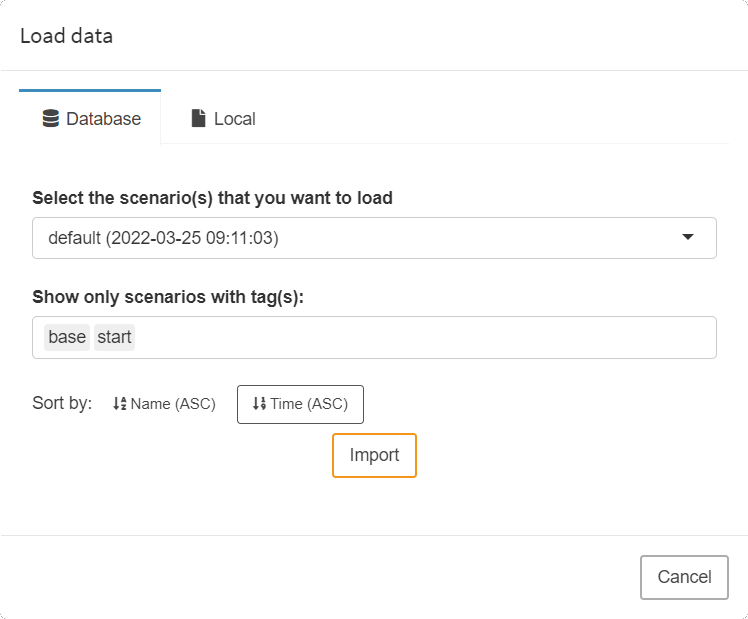
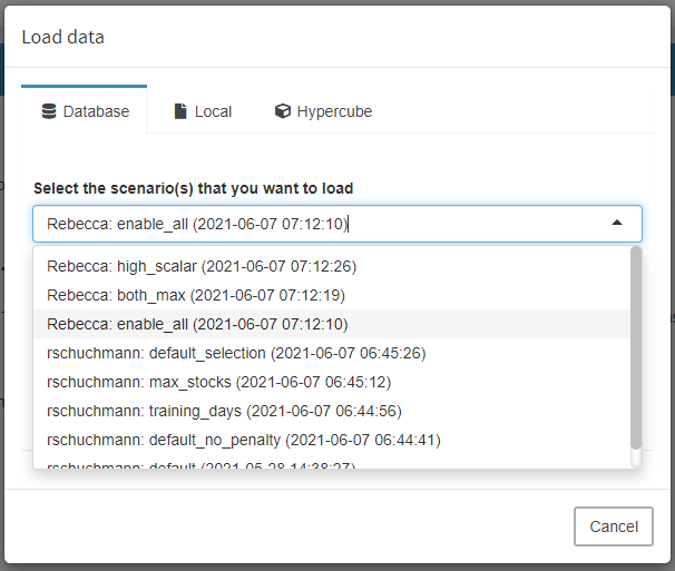
Database Scenarios

Scenarios that you have previously named and saved in the MIRO database will be displayed in Database. When you start a GAMS MIRO app for the first time, GAMS automatically extracts the data from your model and loads this data into the database. This happens every time you rebuild your MIRO app i.e. every time you launch it in the development mode via GAMS Studio or the command line. A special scenario with the name default is created for this purpose and overridden every time you rebuild your app!

Tip:

Every time you start a MIRO app in development mode (via GAMS Studio or the command line), the data relevant to MIRO is extracted from your model and stored in the MIRO database as a special scenario named default.

Local Files

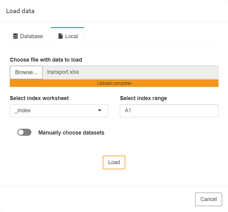
To import a file from your local machine, either in the form of a MIROSCEN file, a GDX container, an Excel spreadsheet or a CSV file, select the menu item Local and click on browse. Navigate to the directory where your file resides and select it. Confirm the data import with a click on import. If you started with an empty sheet, a new, unnamed scenario is now shown in the interface. To save it, click on Save as and give it a name.

Note:

When importing CSV data, delimiters other than the comma are also supported. The currently supported delimiters are: , tab ; | :.

Excel spreadsheet - import rules

If you want to import data from a spreadsheet, it must either contain an index sheet describing the layout of your data, or it must meet certain criteria regarding the format in which the data is provided.

Workbook without index sheet

If you do not want to create an index sheet, your Excel file must meet strict requirements:

Only one GAMS symbol per worksheet
The name of a sheet must be identical to the symbol name
The first line must contain the column headers. The names of the column headers are ignored.
All symbols must be in list view (no columns may be pivoted). The only exceptions to this rule are tables, where the last column must be pivoted.

Either all scalar values are combined in one tab named _scalars or _scalars_out (separate sheets for input and output scalars). These tables must have 3 columns: scalar, description and value.

Alternatively, each scalar value is stored in a separate sheet as with other symbols (tab name = symbol name). The "table" then consists only of the scalar value in cell A1. There is therefore no header.

If you want to import command line parameters/GAMS options, the symbol name must be preceded by _gmspar_ or _gmsopt_ (see screenshot above).
To import scalar output variables and/or equations, the sheet name must be _scalarsve_out. The table has to have 7 columns: scalar, description, level, marginal, lower, upper, scale.

Workbook with index sheet

If you want more flexibility, you must create an index sheet that describes your layout. If you are already familiar with GDXXRW, this will already be familiar to you. You can skip most of this chapter, but be aware of the differences between GDXXRW and MIRO that we list below. We encourage everyone to read the documentation of GDXXRW, especially the chapter about the index option, as it covers the topic in much greater detail than we will do here.

When the layout of your data differs from the default layout described above, you need to tell MIRO where to find what. This can be achieved by a so-called index. Here you list all the GAMS symbols that are included in your workbook as well as the layout they are in.

Note:

Unlike GDXXRW, MIRO already knows a lot about your data from the GAMS/MIRO data contract. This means that information such as the dimensions of your symbols is known to MIRO and does not need to be specified again.

The first three columns of the index range have a fixed interpretation: dataType, symbol identifier and dataRange. Even though MIRO does not need and ignores the dataType information (except dSet, see info box below), it is a good practice to specify it because it allows your worksheet to be read by both MIRO and GDXXRW.

The fourth and subsequent columns can be used for additional options. The column heading indicates the option name and the cell contents indicate the option value. Note that although GDXXRW allows options also in a comma-separated option=value format, MIRO does not support this.

Domain Sets (dSet):

Just like GDXXRW, MIRO supports reading a set as domain set by specifying it as type dSet. This option is supported only for one-dimensional sets. Duplicates and set text are ignored. The dSetText option is also supported by MIRO.

Note that in most cases, it is preferred to use the Implicit Set Definition feature of GAMS! This avoids domain violations caused by having to maintain two tables in MIRO.

Let's look at an example:

The first thing you may notice is the name of the index sheet: _index. Although the index could be on any sheet and in any range, MIRO can automatically recognize it if the sheet is named _index and the index table starts in the upper left corner: A1. The most important information MIRO requires is the symbol name, range (columns B and C) and one of rDim (row dimension) or cDim (column dimension). If neither rDim nor cDim is supplied, MIRO will assume a default of 1 for cDim. This means that the last column is pivoted as is the case for the parameter d:

You can see that the last column (index j) is pivoted. Also note that we can ignore rows and columns via the ignoreRows and ignoreColumns options. In this example, we want to ignore the row 16 because it does not belong to the data for d, but for the set j, which is also read from the same range (sheet1!L15:N16). This brings us to the next option: values. Each tuple in a set can have associated text. To read a set from a spreadsheet, the values option is used to indicate whether there is data, and if so, whether the data should be interpreted as associated text or as an indicator of whether or not the tuple should be included in the set. In our example here, we use the YN option, which specifies that only tuples that have a data cell that is not empty and does not contain 0, N, or No will be included. This means that in our example j only the tuple New-York is read. MIRO supports all options GDXXRW supports: auto, noData, YN, sparse and dense. See the related section of the GDXXRW documentation for more information on the other options. Below you find a list of all options supported by MIRO.

Supported options

Option	Description	Allowed values
range	Excel range: Open and closed ranges are supported. It must be of the form SheetName!TopLeft:BottomRight. If the sheet name is omitted, the first sheet in the workbook is used by default. If the BottomRight corner is omitted, the data is read until `skipEmpty`+1 empty rows/columns are found. If range is omitted, an open range with left upper corner A1 is assumed.
rDim	Row dimension: the number of columns in the data range that will be used to define the labels for the rows. The first rDim columns of the data range will be used for the labels.	0..dim
cDim	Column dimension: the number of rows in the data range that will be used to define the labels for the columns. The first cDim rows of the data range will be used for labels.	0..dim
values	How set data is handled. See the related section of the GDXXRW documentation for more details.	auto, noData, YN, sparse, dense
ignoreRows	Rows to ignore	comma-separated list of positive integers
ignoreColumns	Columns to ignore	comma-separated list of positive integers or column letters
skipEmpty	When reading an open range, controls how many empty rows or columns will be ignored before the next empty row or column indicates the end of the block	0, 1
squeeze	Controls whether zeros are squeezed out/removed	y, 1, n, 0
dSetText	This controls the reading of explanatory text for set elements of domain sets. By default, no text is read for domain sets. If this option is activated this is changed. If an element appears more than once, the first one defines the explanatory text read.	y, 1, n, 0

Reading scalars

In addition to reading each scalar individually as supported by GDXXRW, MIRO also supports reading in table form. To read an entire table of scalars, you must do so using the special _scalars/_scalars_out symbols for input and output scalars, respectively. In this way MIRO reads scalars grouped in a table with 3 columns: Scalar, Description, Value. The Description column can also be omitted. Let's look at our example again:

Layout of individual and grouped scalars

If we look at the corresponding index sheet again, we see that both the output scalar total_cost and the input scalar table _scalars are defined on this sheet. In this example, the table is pivoted (scalar names in the columns) and the Description column has been omitted.

Note that you can mix the declaration of table and individual scalars. Scalars that are missing from the table are appended if they are individually declared. If a scalar is found both in one of the special tables and individually declared, the scalar in the table takes precedence and the individually declared scalar is ignored.

Note:

Command line parameters/GAMS options are treated like normal input scalars with the special prefixes _gmspar_ and _gmsopt_.

Differences between GDXXRW and MIRO

Below we list the important differences you need to be aware of when migrating from GDXXRW to MIRO or vice versa.

Global options are not supported by MIRO: all options are symbol-specific and must be part of the symbol declaration row
The only special values supported by MIRO are: +Inf and -Inf. Eps, YES, NO, NA, Undef, etc. are not properly recognized when used in MIRO
Acronyms are not supported
The only options supported by MIRO are: rDim, cDim, dim, values, ignoreRows, ignoreColumns, skipEmpty, squeeze
Option=value columns are not supported and will be skipped. Please specify the option names as column headers and the values as cell contents.
skipEmpty must be specified for each symbol individually. The state of this option is not transferred to the next symbols as with GDXXRW.
Named ranges are not supported.
Ranges with .. instead of : as separator between TopLeft and BottomRight corner are not supported.
skipEmpty > 1 is not supported i.e. only values 0 and 1 can be used
It is possible to read variables/equations with MIRO. They are treated like normal parameters, with an additional dimension that must contain at least one of the following elements: level, marginal, upper, lower and scale. These do not all have to be assigned, i.e. you can skip some.
When reading scalars, you can either declare them individually as in GDXXRW, or you can use the special symbol names _scalars/_scalars_out to read input/output scalars grouped in a table with 3 columns: Scalar, Description, Value. The Description column can be omitted. You can also mix declaration of individual scalars and scalar tables. Scalars that are missing in the scalar table are appended if they are declared individually. If an individually declared scalar is also in a scalar table, the individually declared scalar is ignored.
In tables/variables/equations, if squeeze=1, empty cells and NA are indistinguishable
Output scalar variables and equations must be in a single table named _scalarsve_out with dimensions: scalar, description, type, where type must not contain any elements other than: level, marginal, upper, lower, scale. Please note that the Description dimension must be present (unlike the _scalars/_scalars_out tables), but is ignored when MIRO imports it.

Instead of importing all the datasets for your model, you can also select the symbols to import manually. To do so, click on Manually choose datasets and choose those symbols to be imported from the uploaded spreadsheet. This will cause MIRO to ignore other datasets.

Import multiple scenarios on startup

In addition to the options mentioned above, which can be accessed directly from MIRO, (multiple) scenarios can also be imported automatically when starting an application. To do this, the scenarios to be imported (MIROSCEN, GDX, CSV or Excel files) must be put in the folder data_<modelname> (located in the model directory). With the next start of MIRO, those scenarios are imported automatically. Note that in development mode MIRO skips the import of files that have not changed since the last start.

In addition to scenario data, views can also be imported together with the scenario data. Simply place the JSON file with the view data here as well. The file has to be named <scenarioName>_views.json. For example if you want to provide data in the form of a GDX file and views for a scenario with the name my_scenario, you have to place both my_scenario.gdx and my_scenario_views.json into the data_<modelname> directory.

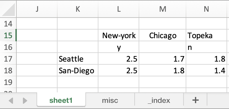
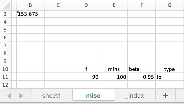
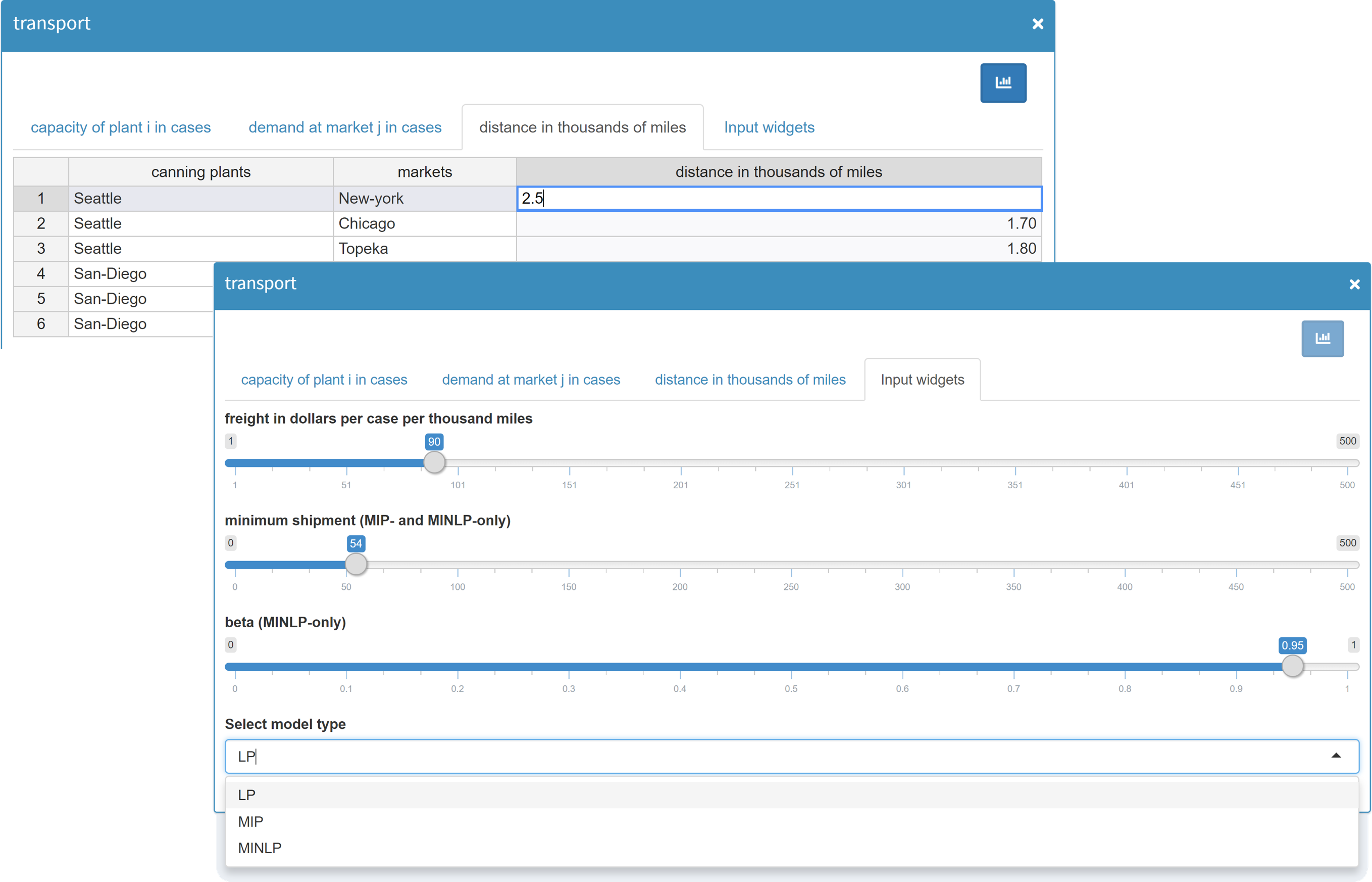
Data manipulation

The tables that were empty before are now populated. In the upper part of the main window, you can navigate between different tabs to switch through the different GAMS symbols that you have specified in your model.
We can now change the input data. You may want to edit individual cells, sort by a different column or add/remove entire records (rows in the table). In our transport demo you have the option to edit the capacities, the demand, the distance matrix and several scalar values:

With the help of sliders and a dropdown menu we can now adjust the freight costs and the model type to be used. If we are satisfied with the settings we can start the GAMS run.

Data cleaning

Your input data must not contain duplicate records. MIRO can help you automatically find and remove duplicate records in your input data sets using the Scenario → Remove duplicates menu in the header. MIRO first checks if any of your input records contain duplicate records, and gives you the option to keep only the first or only the last occurrence of the duplicate.

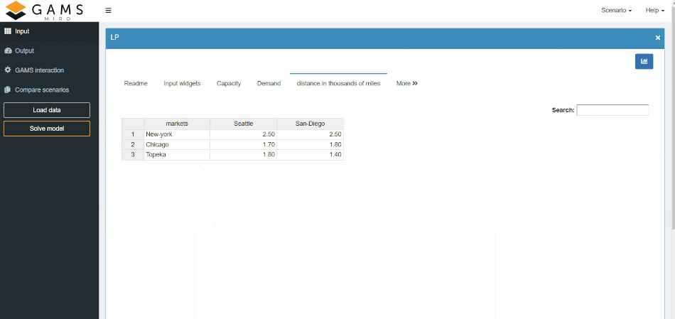
Solve the model

A click on the Solve model button starts the model run. In the background GAMS is called and the model transport.gms is started. The values set by us in MIRO now serve as input data for the model.
During the calculations, MIRO automatically switches to the section GAMS interaction. There you can see the current GAMS log and lst files. If you specified a custom log this is also shown here.

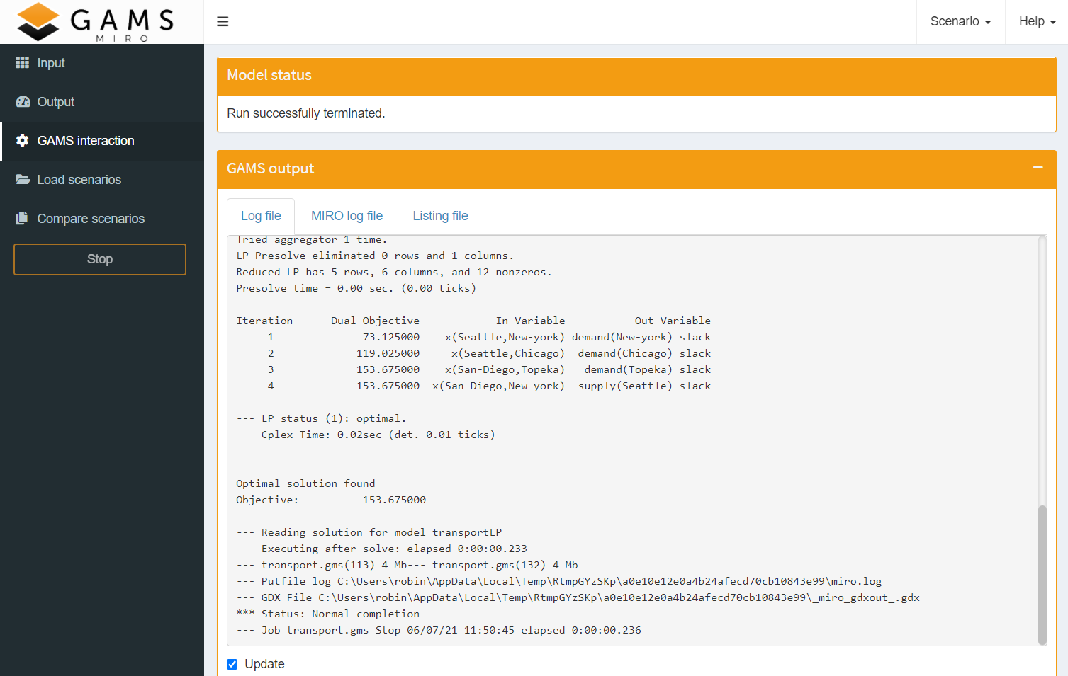
Note: Since the models of the demo applications are solved very quickly, this step is sometimes hardly visible. The menu entry GAMS interaction can also be viewed at any time after a model run.

As long as the calculations are running in GAMS, the Stop button on the left can be clicked. A first click on this button sends an interrupt request to the running job in order to perform a graceful stop and collect an incumbent result back from the execution if the solver supports this feature. A second click sends a request to stop the running job immediately.
After the run, the view changes again to the Output section.

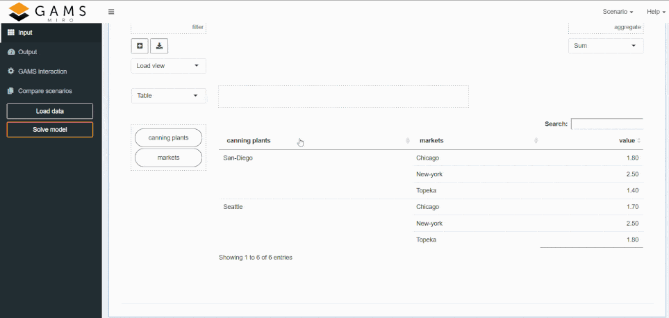
Inspect results

In the Output section the results are visualized. As with the input data, a distinction is made between GAMS parameters and scalar values. The GAMS parameters are each visualized in a separate tab and the scalars are summarized in a table.
If you have configured a graphical representation of your data, you can also see it here. In the model Transport a plot for the transport schedule is configured in the form of a map, see figure below.

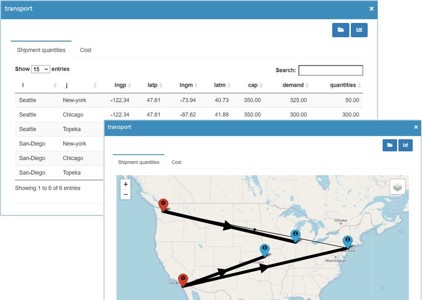
With a click on the button in the upper right corner you can switch between a plot and the tabular representation of the data.

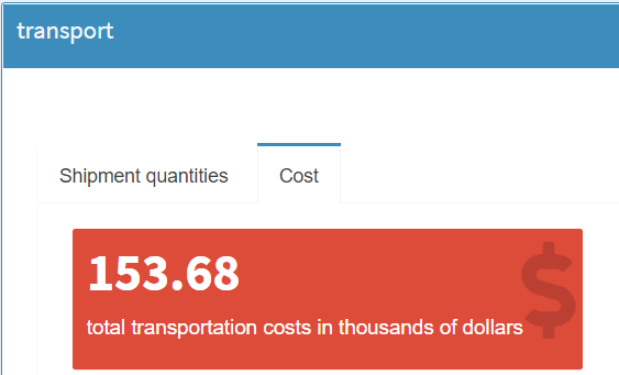
The Costs tab shows the objective function value of the model calculation in a tile. Like before, you can switch between graphical and tabular representation with a click on the button.

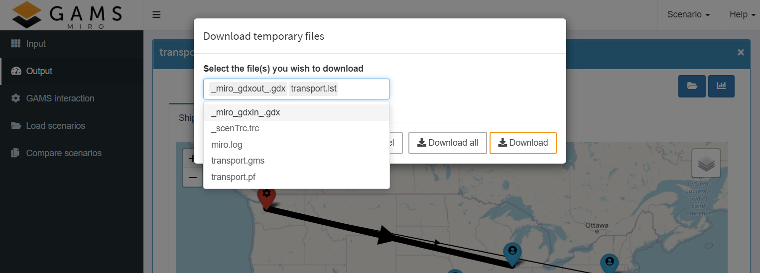
Download temporary files:

If this option is enabled, all temporarily created files of the model run (like solution reports or the lst and log files) can be downloaded either separately or as a ZIP archive with a click on the button.

Save / export / delete a scenario

The set of all the input and output data is what we call a scenario. Data that is currently loaded in the MIRO interface (in memory) is what we call a sandbox scenario (more on this here). A sandbox scenario can be saved at any point. The menu where you can interact with your currently active scenario can be found in header bar of your MIRO app:

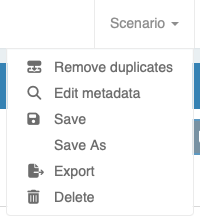
Edit metadata
Allows you to edit scenario metadata, i.e. the scenario name and/or the tags assigned as well as file attachments and scenario access permissions. Read more about scenario metadata here.
Save
Saves the currently active sandbox scenario under an already specified name. Data of the initially loaded scenario is overwritten.

Tip:
Unless otherwise configured, the log and lst file of the GAMS run will also be saved and can be accessed when re-loading the corresponding scenario.
Save As
Saves the currently active sandbox scenario under an new name. If the sandbox scenario has no name yet, only this option is available for saving.

Optionally, you can add tags to the scenario. Tags are stored together with the scenario data. If you want to find a scenario later on, you can search for a given tag. This may help you to better find a certain scenario or a set of scenarios that share certain attributes. Also, if your sandbox scenario contains attachments or you have defined user access permissions, you can adopt these settings for the scenario to be saved.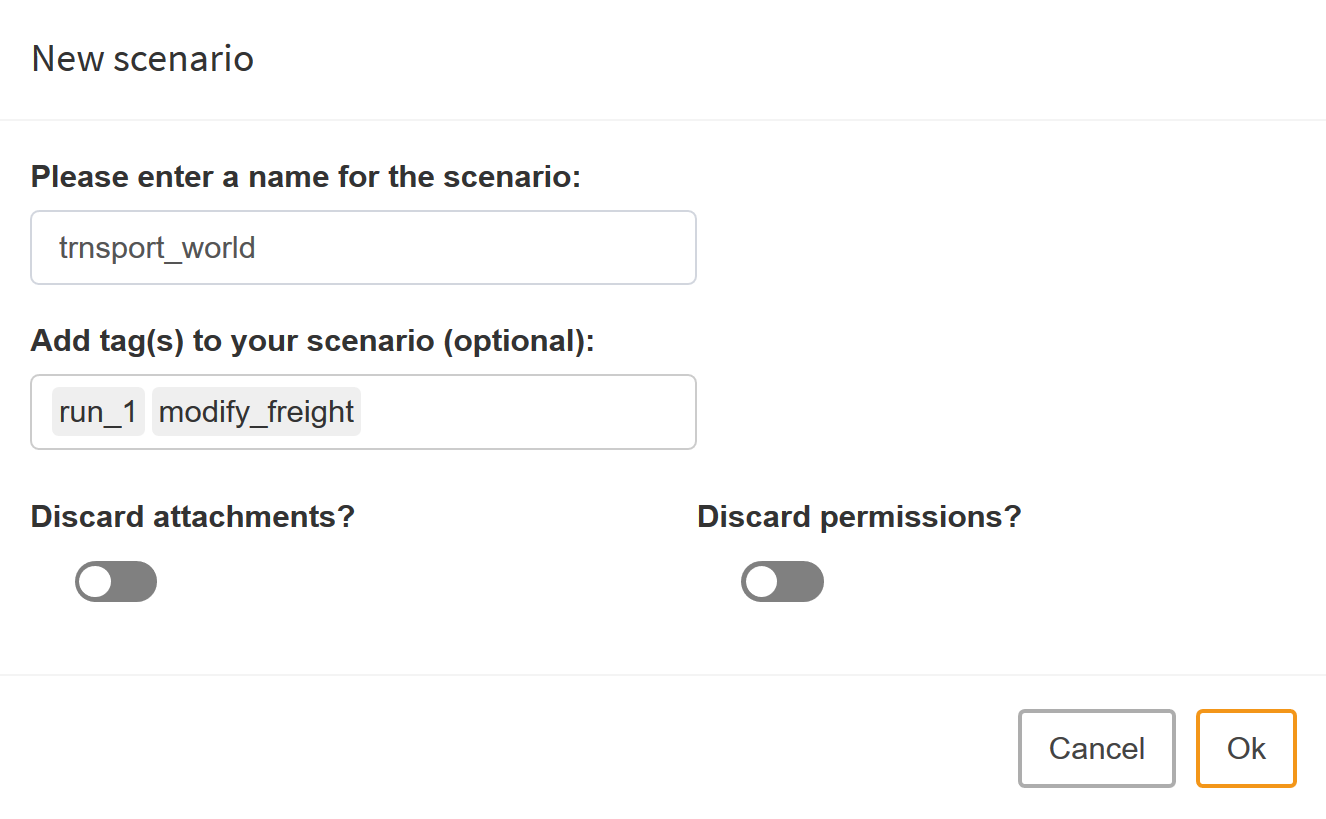
Export
Download of the scenario data in the form of a MIROSCEN file, a GDX container, as an Excel spreadsheet or as CSV files.
Delete
Delete the scenario from the database.

Finding and loading scenarios

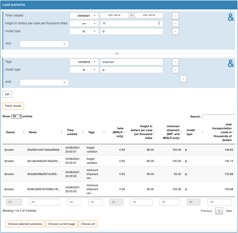
To help you find and load exactly the scenarios you are interested in, MIRO has a powerful Batch Load module that graphically assists you create and execute complex database queries.

Filters can be applied to scenario metadata such as the creation time, scenario name, or optional tags you have assigned to a scenario. You can also filter by any input and output scalars defined in your model as well as any Double-dash parameters and GAMS options. You can combine any of these filters with the logical operators AND and OR:

Tip:

You can search for empty entries (NA) by leaving the field empty if it is a numeric field, or by using the exists and doesn't exist operators for character fields!

You can execute your query by clicking on the Fetch results button. After the results have been retrieved, the page will be updated and you will see a table with the scenarios that correspond to your query.

Results of database search by Batch Load module

Tip:

You can change the name and/or job tag(s) of a scenario by double-clicking the corresponding cell in the table. This can be especially useful for scenarios that were generated via a Hypercube Job and have a (SHA-256) hash as name by default.

Once you have found the scenarios you were looking for, you can do one of the following:

Delete scenarios:
Remove the selected scenarios.
Download data:
Download scenario data for external analysis. Here you can find an example of such an external analysis. The data of selected scenarios were analyzed using R in combination with Jupyter Notebook.
Analyze:
Run one of your customized batch analysis scripts (only visible if you have custom analysis scripts set up).
Load into sandbox:
Load the selected scenario into the sandbox (only visible if you have selected exactly one scenario).
Compare:
Interactive scenario comparison: Compare different scenarios directly in split, tab or pivot view. Best suited for a small number of scenarios to be compared (maximum allowed number of scenarios: 10).

Tip:

When comparing or downloading multiple scenarios, it is sometimes useful to name them according to a common naming scheme based on input/output scalars or other metadata such as creation time. This is especially useful for Hypercube scenarios, since their names are generated automatically. MIRO allows you to choose one or more columns of the Batch Load table to be used for naming scenarios. For example, if we select the "freight Cost" and "minimum shipment" columns to name our scenarios, the first scenario (25E3641B...) in the above image will be named "86_100", the second (da1a8c4b...) will be named "85_100", and so on. As soon as at least one column has been selected for naming the scenarios, another text field appears in which you can additionally specify a (static) prefix for the scenario names.

Scenario comparison

The scenario comparison mode is useful if you want to compare the input and/or output data of different model runs. Scenarios from the database as well as the currently loaded sandbox scenario can be used for comparison. There are three different types of comparison available, split view, tab view and pivot view mode.

Tip:

In case you want to compare multiple scenarios in a different way than the default comparison modes (split view, tab view and pivot view mode) allow, MIRO also supports custom scenario comparison modes.

Pivot view

Unlike the split view and tab view, which take your chart configuration into account, here all records are displayed as pivot tables. Also note that the pivot view comparison mode always compares the sandbox scenario with other scenarios. The sandbox scenario is therefore also called base scenario in this context.

The data of the sandbox scenario and all selected scenarios are merged into a single table with an additional domain: Scenario. You can add/remove scenarios at any time by clicking the button in the upper left corner. To close the scenarios currently loaded in the pivot mode, click the button in the upper right corner. If you have made changes to your sandbox scenario and want to update the data in the pivot view, click the button.

Views can also be used in pivot view mode. They are attached to the sandbox/base scenario. Thus, the scenario you currently have in your sandbox determines what views will be available to you in the pivot view scenario comparison. To save a new view, you only need to save your sandbox scenario once the new view has been added.

Views from the pivot view comparison mode can be managed (imported/exported/deleted) just like normal views via the Views dialog in the Scenario → Edit Metadata menu. You can learn more about views here.

Tip:

If you have opened scenarios in the split or tab view mode and switch to the pivot view, the scenarios from these modes are pre-selected in the load dialog so that you can easily continue using them.

Split view

If two scenarios are to be compared, the split-screen view is particularly suitable. Here the data of two scenarios can be compared side by side.

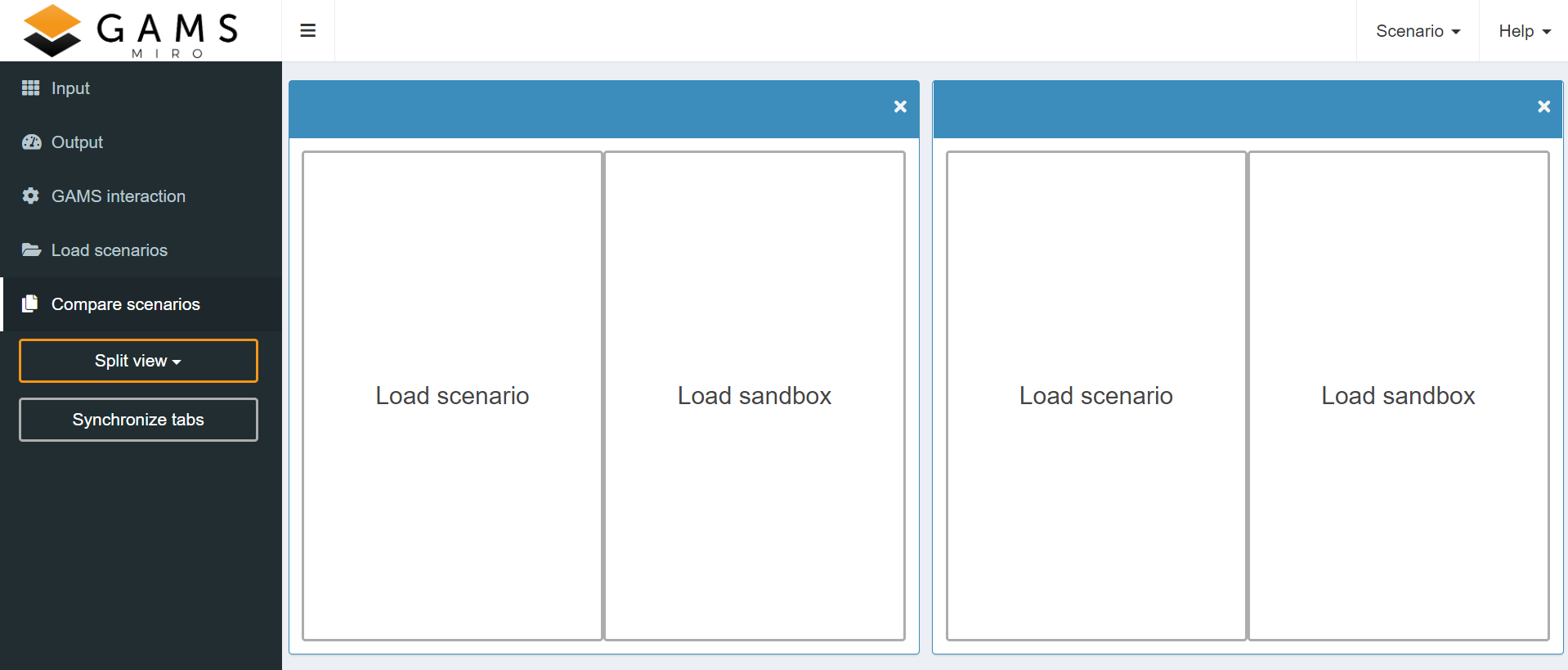
You can choose between:

Load scenario:
Load saved scenario data from the database.
Load sandbox:
Load the sandbox scenario which is opened in the Input / Output section.

Tip:

If you have opened scenarios in the pivot or tab view mode and switch to the split view, the scenarios from these modes are shown in a "Local" tab.

Tab view

Scenarios can also be loaded into tabs (as you know it from e.g. your internet browser). This allows to compare more than two scenarios including their graphics.

Tip:

If you have opened scenarios in the split or pivot view mode and switch to the tab view, the scenarios from these modes are pre-selected in the load dialog so that you can easily continue using them.

Synchronize tabs

The synchronize tabs option makes comparing scenarios more convenient. It can be used in both the split view and the tab view. As soon as this option is activated via the synchronize tabs button in the navigation bar, the switch to another dataset of a scenario is also performed for all other open scenarios. This means that if you change the dataset to be displayed in one scenario (e.g. switch from 'Price' to 'absolute error' in the image above), the view also changes for all the other scenario(s) loaded in the comparison mode.

Tip:

For many operations in MIRO there are shortcuts. Especially when comparing scenarios it can be helpful to switch through the different tabs with shortcuts. You can display all keyboard shortcuts via the command palette. The command palette can be activated by pressing Ctrl+Alt+Space or by navigating to Help → Command palette!

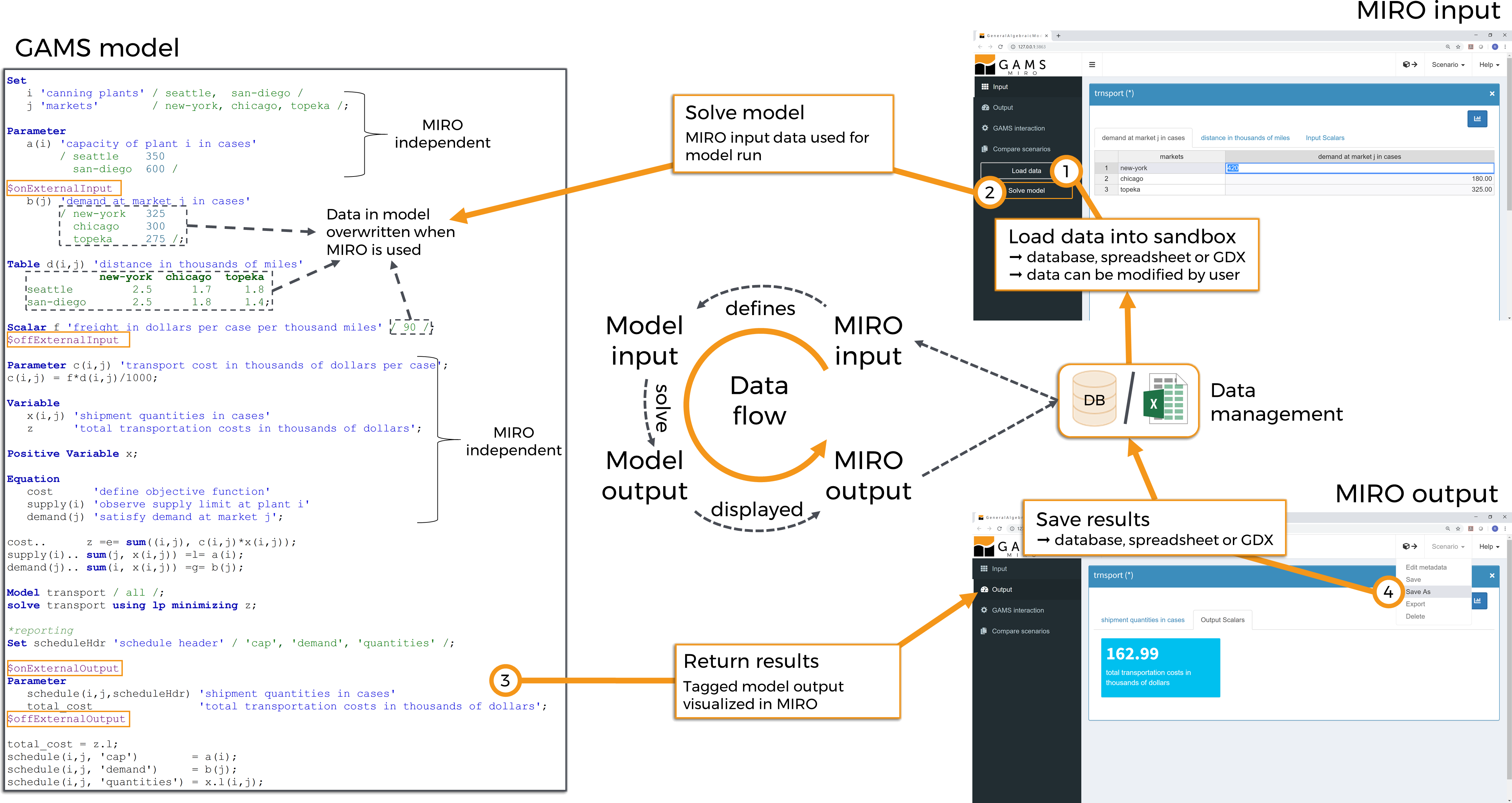
Data concept

To understand the concept of data exchange between the GAMS model and its MIRO application, let's start with the following illustration:

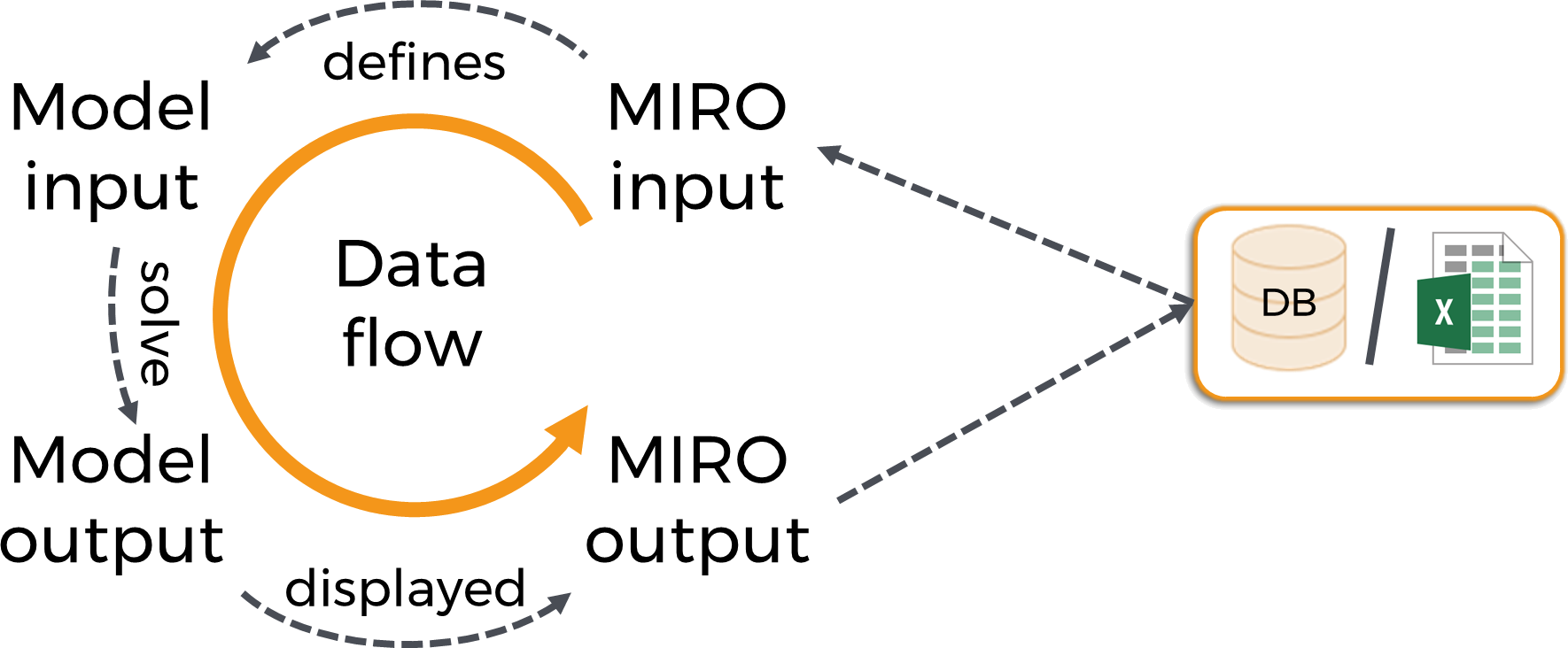
Data is loaded into the MIRO interface. These come either from the internal database, from external data sources such as Excel or GDX or are entered manually, but they do NOT come directly from the GAMS model.
When clicking on solve, the data visible in the MIRO input section is sent to the GAMS model. All data of affected symbols in the model will be overwritten. Symbols that are not visible in MIRO are not touched.
The model is now run with the updated data.
Afterwards the results are sent to MIRO and displayed in the output section. From there, data can be saved in the internal database and/or exported as a file.

A little more detail:

Advanced: Working with NAs, zeros and EPS

Special attention should be paid to the communication of zeros, NAs and EPS between GAMS and MIRO. The following rules describe how the data is communicated in detail:

0:
The data communication between GAMS and MIRO is done via GDX. Zeros are not stored in GDX files. A value of zero in GAMS is therefore not communicated with MIRO and is not visible there. If a GAMS symbol is displayed as a table in MIRO - i.e. the symbol is pivoted by using the table statement or by using the MIRO-side pivoting option - the cells of these missing values are empty.
EPS:
The use of the special value EPS is required when you want to store zeros in a GDX file. In MIRO, a 0 is displayed for the corresponding entries. If a GAMS model is solved out of MIRO, zeros are stored in the GDX file. In the model these can then be interpreted as zeros by using the GAMS option $onEps. If this option is not set, zeros are omitted.
NA:
NAs in GAMS become NAs in MIRO and vice versa. But: NAs are only displayed in the default input tables used in MIRO and only if the table is not pivoted (see above). In output tables (or in input tables where the option to use large amounts of data is enabled), NAs are displayed as blank cells.

Scenario concept

In addition to the data concept, MIRO's scenario concept also needs to be understood.

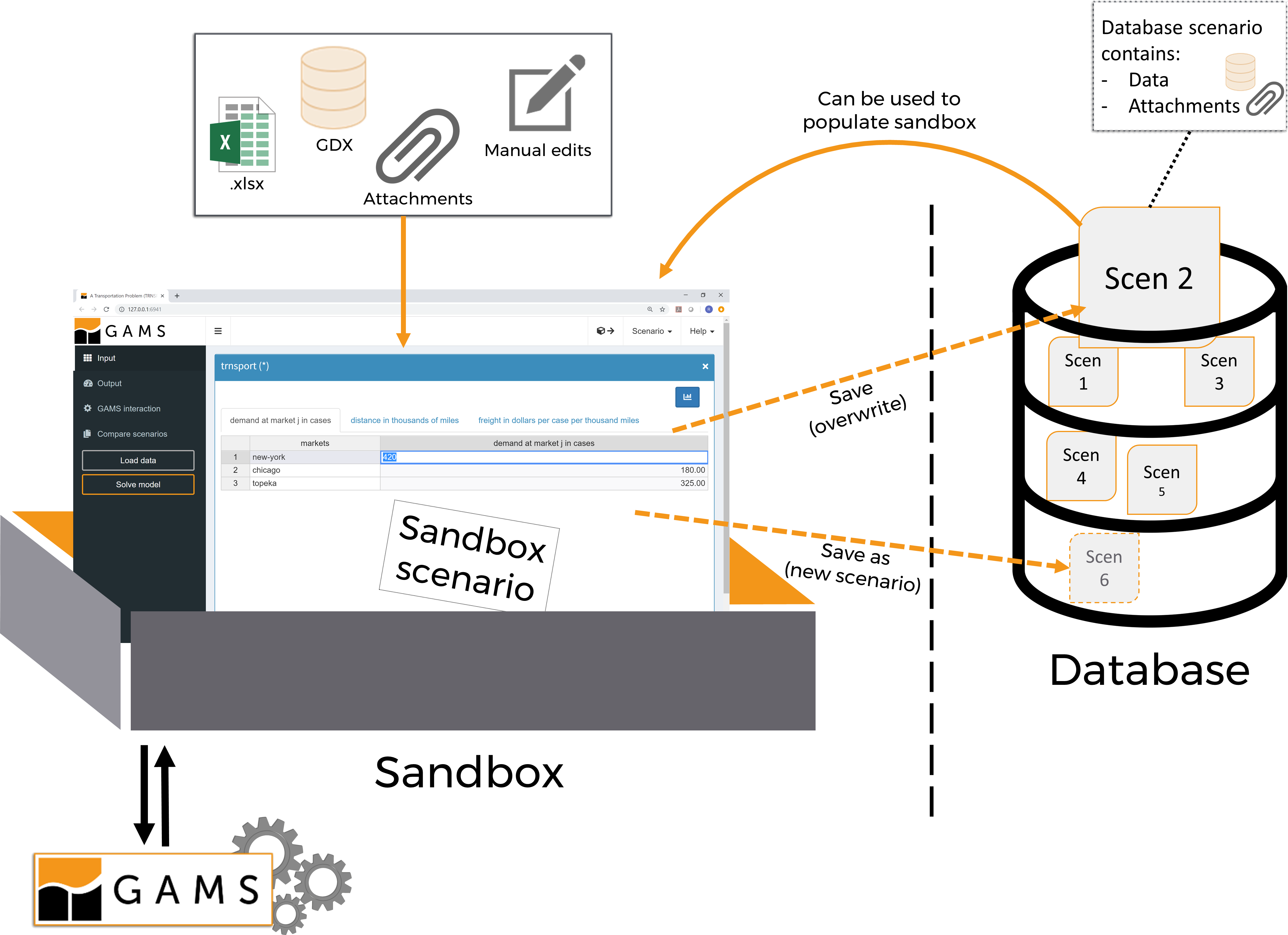
What is a scenario?

We call the collection of input and output datasets that result from a particular model run and which are communicated with MIRO a scenario.
The MIRO user interface can be seen as a sandbox. Data that is loaded into the interface is therefore located in this sandbox as a sandbox scenario.
Scenarios from the database can be loaded into the sandbox. The data of the sandbox scenario can be modified. Data modifications can come from local files or can be entered manually. A click on save overwrites the original scenario in the database with the modified data. Alternatively, a new scenario can be created using save as. The original scenario in the database remains unchanged then.
A sandbox scenario can also be initially created as an empty scenario independent of the database and then filled with data (GDX, Excel, CSV). A scenario created in this way initially does not have a name. As long as a scenario is unnamed, i.e. it is not saved in the database with an individual name, the data is shown exclusively in the interface and gets lost if the MIRO application is closed.
Attachments are part of a scenario. If attachments are added to a sandbox scenario, they are included when saving this scenario.

Scenario metadata

In addition to the classic data of a scenario, which is visualized in the form of tables, widgets and graphics and with which the user interacts primarily for and after a model run, a scenario also consists of metadata. Metadata can be edited under Scenario → Edit metadata. This includes the following:

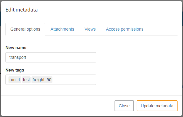
General options

In the general options tab you can change the scenario name and add/edit scenario tags. As mentioned above, you can search for a given tag in the database. Thus, tags can be used to better find a saved scenario or a set of scenarios that share certain attributes.

Attachments

With the attachments option, you can attach files to the (sandbox) scenario you currently have open. These can be files of any format. MIRO distinguishes between attachments that can be seen and read by your GAMS model and files that can not be seen. For example, if you want to provide data to your model that doesn't need to be visible/modifiable in the UI (e.g. in the form of a GDX container or Excel files), attachments that your model can read are what you are looking for. In case you just want to add some report about a particular scenario, which is irrelevant for the GAMS model, you should not allow the model to read this file. Note that all files that you allow your model to read need to be first downloaded into the working directory before GAMS is executed. Thus, it is advisable to select only those files to be readable that are actually relevant for the optimization run.

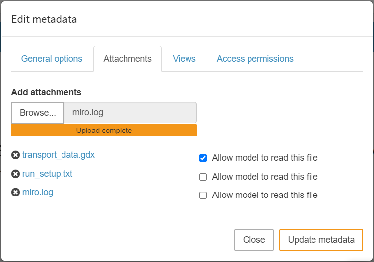
Besides this type of attachments, there are also output attachments which allow you to automatically attach files after a GAMS run has been successfully completed. This lets you store additional results alongside the ones displayed in the UI. You can also use such an attachment for the next GAMS run with this scenario. Read more about output attachments here.

Note:

Attachments added to a sandbox scenario are not automatically saved! If you want to apply the changes to a database scenario, you have to save it.

Views

Views are a special type of attachments that store configurations of renderers. An example is the pivot table renderer. Here a view is a snapshot of the current configuration:

Views can either be bound to a scenario like attachments or registered app-wide. From now on, scenario-specific views will be referred to as local views, while app-wide views will be referred to as global views. You can import and export view configurations in the form of JSON files. Each view has an id that has to be unique per GAMS symbol.

Tip:

Views can also be imported automatically when a MIRO application is started by placing the JSON file(s) in the folder data_<modelname>. Note that views are always tied to a scenario. If you want to store views for a scenario called "my-scenario", you would have a GDX file called my-scenario.gdx as well as a views file called my-scenario_views.json inside the data_<modelname> directory. So the file name of the views must start with the name of the scenario you want to attach them to and end with _views.json.

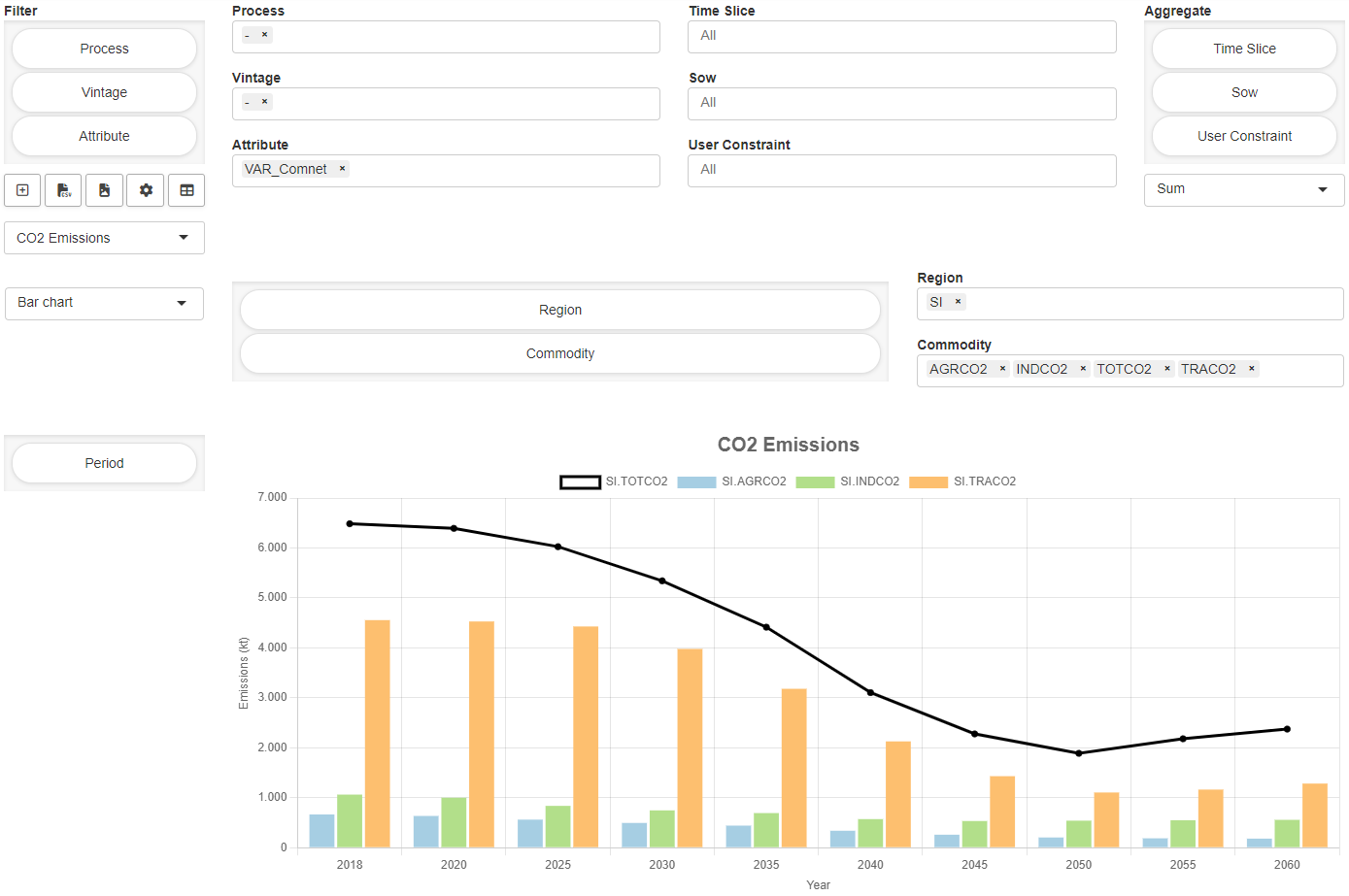
To get a more intuitive understanding of what a view is, the following videos give an example that leads through the most important aspects. With the pivot table renderer, we can filter and aggregate input and output data by dragging and dropping domains. The video below shows how a few actions draw a stacked bar chart of the shipment quantities between canning plants and markets. By clicking the Add View button we can attach a local view to the current scenario. This allows us to return to a configuration later in our analysis.

We can import, download, and remove local views by navigating to the Scenario → Edit metadata → Views dialog. By clicking the Export button, the selected views are saved in the Download folder as a JSON file, which we can use to share with others or to include as global views in the app.

Global views are bundled with a MIRO app and are scenario-independent. A local view can shadow a global view if it has the same name as the global view. This means that when you apply this view, the configuration of the local view is applied. When the local view is removed, the global view is applied again.

Global views can be bundled with an application by placing a JSON file with the filename views.json in the conf_<modelname> directory. This file can also be created automatically by configuring the views via the Configuration Mode.

Access permissions / Scenario sharing

If multiple users have access to the same MIRO app, they can share scenarios. Shared scenarios can be loaded from the database into the sandbox in the same way as your own scenarios.

Since scenario sharing is much more powerful using MIRO Server, you can find more information about this in the MIRO Server section.

Scenario sharing using MIRO Desktop:
Scenarios can also be shared in MIRO Desktop. However, unlike MIRO Server, MIRO Desktop does not offer sophisticated user management including user groups. Users of a local MIRO Desktop application are automatically assigned to the only group available, 'users'. As a consequence, scenarios can be shared either with all users ('users' group) or with no users.

Note:

In contrast to the database used by GAMS MIRO Server, the database for MIRO Desktop is not designed for concurrent use. We therefore recommend to use one database per user for MIRO Desktop applications.

Performance Aspects

The size and/or complexity of a GAMS model does not affect the performance of a MIRO application. As the data concept shows, only data declared as external input and output (data contract) is communicated between the model and the application. The amount of data to be exchanged as well as the complexity of its visualization influence the performance of your application. Important factors are:

Number of symbols that are communicated with MIRO
The more symbols you want to display in MIRO, the more tables and charts need to be set up. MIRO renders most of them lazily, that is, only when the user actually activates a particular tab. However, each of the symbols has a slight overhead and you should ask yourself whether displaying all of them is really necessary. For example, it is usually not a good idea to declare each domain set separately as external input. Instead, use the Implicit Set Definition feature of GAMS! This not only saves rendering time in MIRO, but is often better for the user experience as it simplifies data entry. As a rule of thumb, try to limit the number of symbols in your data contract to 50.
Amount of data that is communicated with MIRO
Each dataset is displayed in MIRO in the form of a table and a graph. The larger the amount of data, the more computationally intensive this process becomes. In addition, the rendering of graphics can vary in complexity. While a simple pie chart is usually rendered fairly quickly, graphs that contain animations can take significantly more time. In the case of very large amounts of data that are only displayed in MIRO for visualization purposes, it may make sense from a performance point of view to communicate only parts of the data with MIRO or to visualize only sections of it, e.g. by aggregating data.
Table tool to use
MIRO provides several table tools for input symbols, each of which has its advantages and disadvantages. The default input data tool provides a spreadsheet-like feel. However, all data is held in the user's browsers, which becomes problematic when dealing with large amounts of data. If you have larger data sets (>10,000 records and >10 columns), MIRO offers the Big Data Table as well as the MIRO Pivot Table. With these two table types, most of the data is kept on the server side and only fractions of the data are kept in the user's browser. This allows for much larger data sets (>3 million records).
Attachments provide a convenient way to communicate large amounts of data from MIRO to the GAMS model without significantly impacting application performance. Since attachments are communicated as a file and therefore do not require data to be rendered, they require very few computational resources.

What's Next

If you are using an existing MIRO application, you are now ready to work with input data, execute optimization jobs, manage scenarios, and analyze results.

If you do not have a MIRO application yet, the next step is to prepare your own GAMS or GAMSPy model for MIRO. The Model Preparation guide explains how to define the MIRO data contract and transform a model into a fully functional MIRO application.