Table of Contents
Complementarity
A fundamental problem of mathematics is to find a solution to a square system of nonlinear equations. Two generalizations of nonlinear equations have been developed, a constrained nonlinear system which incorporates bounds on the variables, and the complementarity problem (MCP). This document is primarily concerned with the complementarity problem.
The PATH solver for MCP models is a Newton-based solver that combines a number of the most effective variations, extensions, and enhancements of this powerful technique. See PATH vs MILES for a comparison with MILES. Algorithmic details can also be found in papers and technical reports by Dirkse, Ferris, and Munson on Ferris' Home Page.
The complementarity problem adds a combinatorial twist to the classic square system of nonlinear equations, thus enabling a broader range of situations to be modeled. In its simplest form, the combinatorial problem is to choose from \(2n\) inequalities a subset of \(n\) that will be satisfied as equations. These problems arise in a variety of disciplines including engineering and economics [59] where we might want to compute Wardropian and Walrasian equilibria, and optimization where we can model the first order optimality conditions for nonlinear programs [102, 114] . Other examples, such as bimatrix games [117] and options pricing [97] , abound.
Our development of complementarity is done by example. We begin by looking at the optimality conditions for a transportation problem and some extensions leading to the nonlinear complementarity problem. We then discuss a Walrasian equilibrium model and use it to motivate the more general mixed complementarity problem. We conclude this chapter with information on solving the models using the PATH solver and interpreting the results.
Transportation Problem
The transportation model is a linear program where demand for a single commodity must be satisfied by suppliers at minimal transportation cost. The underlying transportation network is given as a set \(\mathcal{A}\) of arcs, where \((i,j) \in \mathcal{A}\) means that there is a route from supplier \(i\) to demand center \(j\). The problem variables are the quantities \(x_{i,j}\) shipped over each arc \((i,j)\in \mathcal{A}\). The linear program can be written mathematically as
\begin{equation} \tag{1} \begin{array}{rc} \min_{x \geq 0} & \sum_{(i,j) \in \mathcal{A}} c_{i,j} x_{i,j} \\ \mbox{subject to} & \sum_{j: (i,j) \in \mathcal{A}} x_{i,j} \leq s_i, \;\forall i \\ & \sum_{i: (i,j) \in \mathcal{A}} x_{i,j} \geq d_j, \;\forall j. \end{array} \end{equation}
where \(c_{i,j}\) is the unit shipment cost on the arc \((i,j)\), \(s_i\) is the available supply at \(i\), and \(d_j\) is the demand at \(j\).
The derivation of the optimality conditions for this linear program begins by associating with each constraint a multiplier, alternatively termed a dual variable or shadow price. These multipliers represent the marginal price on changes to the corresponding constraint. We label the prices on the supply constraint \(p^s\) and those on the demand constraint \(p^d\). Intuitively, for each supply node \(i\)
\[ 0 \leq p^s_i, \; s_i \geq \sum_{j: (i,j) \in \mathcal{A}} x_{i,j}. \]
Consider the case when \(s_i > \sum_{j: (i,j) \in \mathcal{A}} x_{i,j}\), that is there is excess supply at \(i\). Then, in a competitive marketplace, no rational person is willing to pay for more supply at node \(i\); it is already over-supplied. Therefore, \(p^s_i = 0\). Alternatively, when \(s_i = \sum_{j: (i,j) \in \mathcal{A}} x_{i,j}\), that is node \(i\) clears, we might be willing to pay for additional supply of the good. Therefore, \(p^s_i \geq 0\). We write these two conditions succinctly as:
\[ \begin{array}{rcll} 0 \leq p^s_i & \perp & s_i \geq \sum_{j: (i,j) \in \mathcal{A}} x_{i,j}, & \forall i \end{array} \]
where the \(\perp\) notation is understood to mean that at least one of the adjacent inequalities must be satisfied as an equality. For example, either \(0 = p^s_i\), the first case, or \(s_i = \sum_{j: (i,j) \in \mathcal{A}} x_{i,j}\), the second case.
Similarly, at each node \(j\), the demand must be satisfied in any feasible solution, that is
\[ \sum_{i: (i,j) \in \mathcal{A}} x_{i,j} \geq d_j. \]
Furthermore, the model assumes all prices are nonnegative, \(0 \leq p^d_j\). If there is too much of the commodity supplied, \(\sum_{i: (i,j) \in \mathcal{A}} x_{i,j} > d_j\), then, in a competitive marketplace, the price \(p^d_j\) will be driven down to \(0\). Summing these relationships gives the following complementarity condition:
\[ \begin{array}{rcll} 0 \leq p^d_j & \perp & \sum_{i: (i,j) \in \mathcal{A}} x_{i,j} \geq d_j, & \forall j . \end{array} \]
The supply price at \(i\) plus the transportation cost \(c_{i,j}\) from \(i\) to \(j\) must exceed the market price at \(j\). That is, \(p^s_i + c_{i,j} \geq p^d_j\). Otherwise, in a competitive marketplace, another producer will replicate supplier \(i\) increasing the supply of the good in question which drives down the market price. This chain would repeat until the inequality is satisfied. Furthermore, if the cost of delivery strictly exceeds the market price, that is \(p^s_i + c_{i,j} > p^d_j\), then nothing is shipped from \(i\) to \(j\) because doing so would incur a loss and \(x_{i,j} = 0\). Therefore,
\[ \begin{array}{rcll} 0 \leq x_{i,j} & \perp & p^s_i + c_{i,j} \geq p^d_j, & \forall (i,j) \in \mathcal{A}. \end{array} \]
We combine the three conditions into a single problem,
\begin{equation} \tag{2} \begin{array}{rcll} 0 \leq p^s_i & \perp & s_i \geq \sum_{j: (i,j) \in \mathcal{A}} x_{i,j}, & \forall i \\ 0 \leq p^d_j & \perp & \sum_{i: (i,j) \in \mathcal{A}} x_{i,j} \geq d_j, & \forall j \\ 0 \leq x_{i,j} & \perp & p^s_i + c_{i,j} \geq p^d_j, & \forall (i,j) \in \mathcal{A}. \end{array} \end{equation}
This model defines a linear complementarity problem that is easily recognized as the complementary slackness conditions [36] of the linear program (1). For linear programs the complementary slackness conditions are both necessary and sufficient for \(x\) to be an optimal solution of the problem (1). Furthermore, the conditions (2) are also the necessary and sufficient optimality conditions for a related problem in the variables \((p^s,p^d)\)
\[ \begin{array}{rc} \max_{p^s,p^d \geq 0} & \sum_j d_j p^d_j - \sum_i s_i p^s_i \\ \mbox{subject to} & c_{i,j} \geq p^d_j - p^s_i, \; \forall (i,j) \in \mathcal{A} \end{array} \]
termed the dual linear program (hence the nomenclature "dual variables").
Looking at (2) a bit more closely we can gain further insight into complementarity problems. A solution of (2) tells us the arcs used to transport goods. A priori we do not need to specify which arcs to use, the solution itself indicates them. This property represents the key contribution of a complementarity problem over a system of equations. If we know what arcs to send flow down, we can just solve a simple system of linear equations. However, the key to the modeling power of complementarity is that it chooses which of the inequalities in (2) to satisfy as equations. In economics we can use this property to generate a model with different regimes and let the solution determine which ones are active. A regime shift could, for example, be a back stop technology like windmills that become profitable if a \(CO_2\) tax is increased.
GAMS Code
The GAMS code for the complementarity version of the transportation problem is given in Figure 1; the actual data for the model is assumed to be given in the file transmcp.dat. Note that the model written corresponds very closely to (2). In GAMS, the \(\perp\) sign is replaced in the model statement with a ".". It is precisely at this point that the pairing of variables and equations shown in (2) occurs in the GAMS code. For example, the function defined by rational is complementary to the variable x. To inform a solver of the bounds, the standard GAMS statements on the variables can be used, namely (for a declared variable \(z(i)\)):
z.lo(i) = 0;
or alternatively
positive variable z;
Further information on the GAMS syntax can be found in [155]. Note that GAMS requires the modeler to write F(z) =g= 0 whenever the complementary variable is lower bounded, and does not allow the alternative form 0 =l= F(z).
Figure 1: A simple MCP model in GAMS, transmcp.gms
sets   i   canning plants,
       j   markets ;

parameter
       s(i)    capacity of plant i in cases,
       d(j)    demand at market j in cases,
       c(i,j)  transport cost in thousands of dollars per case ;

$include transmcp.dat

positive variables
       x(i,j)           shipment quantities in cases
       p_demand(j)      price at market j
       p_supply(i)      price at plant i;

equations
       supply(i)      observe supply limit at plant i
       demand(j)      satisfy demand at market j
       rational(i,j);

supply(i) ..     s(i) =g= sum(j, x(i,j)) ;

demand(j) ..     sum(i, x(i,j))  =g=  d(j) ;

rational(i,j) .. p_supply(i) + c(i,j) =g= p_demand(j) ;

model transport / rational.x, demand.p_demand, supply.p_supply /;

solve transport using mcp;
Extension: Model Generalization
While many interior point methods for linear programming exploit this complementarity framework (so-called primal-dual methods [203] ), the real power of this modeling format is the new problem instances it enables a modeler to create. We now show some examples of how to extend the simple model (2) to investigate other issues and facets of the problem at hand.
Demand in the model of Figure 1 is independent of the prices \(p\). Since the prices \(p\) are variables in the complementarity problem (2), we can easily replace the constant demand \(d\) with a function \(d(p)\) in the complementarity setting. Clearly, any algebraic function of \(p\) that can be expressed in GAMS can now be added to the model given in Figure 1. For example, a linear demand function could be expressed using
\[ \sum_{i: (i,j) \in \mathcal{A}} x_{i,j} \geq d_j(1-p^d_j),\; \forall j. \]
Note that the demand is rather strange if \(p^d_j\) exceeds 1. Other more reasonable examples for \(d(p)\) are easily derived from Cobb-Douglas or CES utilities. For those examples, the resulting complementarity problem becomes nonlinear in the variables \(p\). Details of complementarity for more general transportation models can be found in [46] , [61] .
Another feature that can be added to this model are tariffs or taxes. In the case where a tax is applied at the supply point, the third general inequality in (2) is replaced by
\[ p^s_i ( 1 + t_i ) + c_{i,j} \geq p^d_j,\; \forall (i,j) \in \mathcal{A}. \]
The taxes can be made endogenous to the model, details are found in [155] .
The key point is that with either of the above modifications, the complementarity problem is not just the optimality conditions of a linear program. In many cases, there is no optimization problem corresponding to the complementarity conditions.
Nonlinear Complementarity Problem
We now abstract from the particular example to describe more carefully the complementarity problem in its mathematical form. All the above examples can be cast as nonlinear complementarity problems (NCPs) defined as follows:
(NCP) Given a function \(F : \mathbf{R}^{n} \rightarrow \mathbf{R}^{n}\), find \(z \in \mathbf{R}^n\) such that
\[ 0 \leq z \perp F(z) \geq 0. \]
Recall that the \(\perp\) sign signifies that one of the inequalities is satisfied as an equality, so that componentwise, \(z_iF_i(z) = 0\). We frequently refer to this property as \(z_i\) is complementary to \(F_i\). A special case of the NCP that has received much attention is when \(F\) is a linear function, the linear complementarity problem [39] .
Walrasian Equilibrium
A Walrasian equilibrium can also be formulated as a complementarity problem (see [132] ). In this case, we want to find a price \(p \in \mathbf{R}^m\) and an activity level \(y \in \mathbf{R}^n\) such that
\begin{equation} \tag{3} \begin{array}{rclcr} 0 \leq y & \perp & L(p) & := & -A^T p \geq 0 \\ 0 \leq p & \perp & S(p,y) & := & b + Ay - d(p) \geq 0 \end{array} \end{equation}
where \(S(p,y)\) represents the excess supply function and \(L(p)\) represents the loss function. Complementarity allows us to choose the activities \(y_j\) to run (i.e. only those that do not make a loss). The second set of inequalities state that the price of a commodity can only be positive if there is no excess supply. These conditions indeed correspond to the standard exposition of Walras' law which states that supply equals demand if we assume all prices \(p\) will be positive at a solution. Formulations of equilibria as systems of equations do not allow the model to choose the activities present, but typically make an a priori assumption on this matter.
GAMS Code
A GAMS implementation of (3) is given in Figure 2. Many large scale models of this nature have been developed. An interested modeler could, for example, see how a large scale complementarity problem was used to quantify the effects of the Uruguay round of talks [94] .
Figure 2: Walrasian equilibrium as an NCP, walras1.gms
$include walras.dat

positive variables p(i), y(j);
equations S(i), L(j);

S(i)..   b(i) + sum(j, A(i,j)*y(j)) - c(i)*sum(k, g(k)*p(k)) / p(i)
         =g= 0;

L(j)..   -sum(i, p(i)*A(i,j)) =g= 0;

model walras / S.p, L.y /;
solve walras using mcp;
Extension: Intermediate Variables
In many modeling situations, a key tool for clarification is the use of intermediate variables. As an example, the modeler may wish to define a variable corresponding to the demand function \(d(p)\) in the Walrasian equilibrium (3). The syntax for carrying this out is shown in Figure 3 where we use the variables d to store the demand function referred to in the excess supply equation. The model walras now contains a mixture of equations and complementarity constraints. Since constructs of this type are prevalent in many practical models, the GAMS syntax allows such formulations.
Figure 3: Walrasian equilibrium as an MCP, walras2.gms
$include walras.dat

positive variables p(i), y(j);
variables d(i);
equations S(i), L(j), demand(i);

demand(i)..
         d(i) =e= c(i)*sum(k, g(k)*p(k)) / p(i) ;

S(i)..   b(i) + sum(j, A(i,j)*y(j)) - d(i) =g= 0 ;

L(j)..   -sum(i, p(i)*A(i,j)) =g= 0 ;

model walras / demand.d, S.p, L.y /;
solve walras using mcp;
Note that positive variables are paired with inequalities, while free variables are paired with equations. A crucial point misunderstood by many modelers (new and experienced alike) is that the bounds on the variable determine the relationships satisfied by the function \(F\). Thus in Figure 3, \(d\) is a free variable and therefore its paired equation demand is an equality. Similarly, since \(p\) is nonnegative, its paired relationship S is a (greater-than) inequality. See the MCP definition below for details.
A simplification is allowed to the model statement in Figure 3. It is not required to match free variables explicitly to equations; we only require that there are the same number of free columns (i.e. single variables) as unmatched rows (i.e. single equations). Thus, in the example of Figure 3, the model statement could be replaced by
model walras / demand, S.p, L.y /;
This extension allows existing GAMS models consisting of a square system of nonlinear equations to be easily recast as a complementarity problem - the model statement is unchanged. GAMS generates a list of all variables appearing in the equations found in the model statement, performs explicitly defined pairings and then checks that the number of remaining equality rows equals the number of remaining free columns. However, if an explicit match is given, the PATH solver can frequently exploit the information for better solution. Note that all variables that are not free and all inequalities must be explicitly matched.
Mixed Complementarity Problem
A mixed complementarity problem (MCP) is specified by three pieces of data, namely the lower bounds \(\ell\), the upper bounds \(u\) and the function \(F\).
(MCP) Given lower bounds \(\ell \in \{ \mathbf{R}\cup\{-\infty\}\}^n\), upper bounds \(u \in \{ \mathbf{R}\cup\{\infty\}\}^n\) and a function \(F: \mathbf{R}^n \rightarrow \mathbf{R}^n\), find \(z \in \mathbf{R}^n\) such that precisely one of the following holds for each \(i \in \{1, \ldots, n\}\):
\[ \begin{array}{rcl} F_i(z) = 0 & \mbox{ and } & \ell_i \leq z_i \leq u_i \\ F_i(z) > 0 & \mbox{ and } & z_i = \ell_i \\ F_i(z) < 0 & \mbox{ and } & z_i = u_i . \end{array} \]
These relationships define a general MCP (sometimes termed a rectangular variational inequality [93] ). We will write these conditions compactly as
\[ \begin{array}{rcl} \ell \leq x \leq u & \perp & F(x). \end{array} \]
As the MCP model type as defined above is the one used in GAMS, there are some consequences of the definition worth emphasizing here. Firstly, the bounds on the variable determine the relationships satisfied by the function \(F\): the constraint type (e.g. =G=, =L=) chosen plays no role in defining the problem. This being the case, it is acceptable (and perhaps advisable!) to use an =N= in the definition of all equations used in complementarity models to highlight the dependence on the variable bounds in defining the MCP. This is not required, however. The constraint types =G=, =L= and =E= are also allowed. If the variable bounds are inconsistent with the constraint type chosen, GAMS will either reject the model (e.g. an =L= row matched with a lower-bounded variable) or silently and temporarily ignore the issue (e.g. an =E= row matched with a lower-bounded variable). In the latter case, if equality does not hold at solution (allowable if the variable is at lower bound) the is marked in the listing file with a redef.
Secondly, note the contrast between complementarity conditions like \(g(z) \leq 0, z \geq 0\) and a complementarity problem like \(F(x) \ \perp \ 0 \leq x \leq \infty\). The former requires a trivial transformation in order to fit into the MCP framework: \(-g(z) \ \perp \ 0 \leq z \leq \infty\). This simple issue is a frequent source of problems and worth looking out for.
The nonlinear complementarity problem of Nonlinear Complementarity Problem is a special case of the MCP. For example, to formulate an NCP in the GAMS/MCP format we set
z.lo(I) = 0;
or declare
positive variable z;
Another special case is a square system of nonlinear equations
(NE) Given a function \(F : \mathbf{R}^{n} \rightarrow \mathbf{R}^{n}\) find \(z \in \mathbf{R}^n\) such that
\[ F(z) = 0. \]
In order to formulate this in the GAMS/MCP format we just declare
free variable z;
In both the above cases, we must not modify the lower and upper bounds on the variables later (unless we wish to drastically change the problem under consideration).
An advantage of the extended formulation described above is the pairing between "fixed" variables (ones with equal upper and lower bounds) and a component of \(F\). If a variable \(z_i\) is fixed, then \(F_i(z)\) is unrestricted since precisely one of the three conditions in the MCP definition automatically holds when \(z_i = \ell_i = u_i\). Thus if a variable is fixed in a GAMS model, the paired equation is completely dropped from the model. This convenient modeling trick can be used to remove particular constraints from a model at generation time. As an example, in economics, fixing a level of production will remove the zero-profit condition for that activity.
Simple bounds on the variables are a convenient modeling tool that translates into efficient mathematical programming tools. For example, specialized codes exist for the bound constrained optimization problem
\[ \min f(x) \mbox{ subject to } \ell \leq x \leq u . \]
The first order optimality conditions for this problem class are precisely MCP( \(\nabla f(x), [\ell,u]\)). We can easily see this condition in a one dimensional setting. If we are at an unconstrained stationary point, then \(\nabla f(x) = 0\). Otherwise, if \(x\) is at its lower bound, then the function must be increasing as \(x\) increases, so \(\nabla f(x) \geq 0\). Conversely, if \(x\) is at its upper bound, then the function must be increasing as \(x\) decreases, so that \(\nabla f(x) \leq 0\). The MCP allows such problems to be easily and efficiently processed.
Upper bounds can be used to extend the utility of existing models. For example, in Figure 3 it may be necessary to have an upper bound on the activity level \(y\). In this case, we simply add an upper bound to \(y\) in the model statement, and we can replace the loss equation with the following definition:
     y.up(j) = 10;
     L(j)..   -sum(i, p(i)*A(i,j)) =e= 0 ;
Here, for bounded variables, we do not know beforehand if the constraint will be satisfied as an equation, less-than inequality or greater-than inequality, since this determination depends on the values of the solution variables. However, let us interpret the relationships that the above change generates. If \(y_j = 0\), the loss function can be positive since we are not producing in the \(j\)th sector. If \(y_j\) is strictly between its bounds, then the loss function must be zero by the definition of complementarity; this is the competitive assumption. Finally, if \(y_j\) is at its upper bound, then the loss function can be negative. Of course, if the market does not allow free entry, some firms may operate at a profit (negative loss). For more examples of problems, the interested reader is referred to [43] , [58] , [59] .
Solution
We will assume that a file named transmcp.gms has been created using the GAMS syntax which defines an MCP model transport as developed in Transportation Problem . The modeler has a choice of the complementarity solver to use. We are going to further assume that the modeler wants to use PATH.
There are two ways to ensure that PATH is used as opposed to any other GAMS/MCP solver. These are as follows:
- Add the following line to the
transmcp.gmsfile prior to thesolvestatementoption mcp = path;
PATH will then be used instead of the default solver provided. - Choose PATH as the default solver for MCP (via a gamsconfig.yaml file or by rerunning
gamsinstfrom the GAMS system directory).
To solve the problem, the modeler executes the command:
gams transmcp
where transmcp can be replaced by any filename containing a GAMS model. Many other command line options for GAMS exist; the reader is referred to List of Command Line Parameters for further details.
At this stage, control is handed over to the solver which creates a log providing information on what the solver is doing as time elapses. See Section PATH for details about the log file. After the solver terminates, a listing file is generated containing the solution to the problem. We now describe the listing file output specifically related to complementarity problems.
Listing File
The listing file is the standard GAMS mechanism for reporting model results. This file contains information regarding the compilation process, the form of the generated equations in the model, and a report from the solver regarding the solution process.
We now detail the last part of this output, an example of which is given in Figure 4 . We use "..." to indicate where we have omitted continuing similar output.
Figure 4: Listing File for solving transmcp.gms
              S O L V E      S U M M A R Y

     MODEL   TRANSPORT
     TYPE    MCP
     SOLVER  PATH                FROM LINE  45

**** SOLVER STATUS     1 NORMAL COMPLETION
**** MODEL STATUS      1 OPTIMAL

 RESOURCE USAGE, LIMIT          0.057     1000.000
 ITERATION COUNT, LIMIT        31        10000
 EVALUATION ERRORS              0            0

 Work space allocated           --    0.06 Mb


---- EQU RATIONAL

                      LOWER     LEVEL     UPPER    MARGINAL

seattle  .new-york    -0.225    -0.225     +INF     50.000
seattle  .chicago     -0.153    -0.153     +INF    300.000
seattle  .topeka      -0.162    -0.126     +INF       .

...

---- VAR X           shipment quantities in cases

                      LOWER     LEVEL     UPPER    MARGINAL

seattle  .new-york      .       50.000     +INF       .
seattle  .chicago       .      300.000     +INF       .

...

**** REPORT SUMMARY :        0     NONOPT
                             0 INFEASIBLE
                             0  UNBOUNDED
                             0  REDEFINED
                             0     ERRORS
After a summary line indicating the model name and type and the solver name, the listing file shows a solver status and a model status. Table 1 and Table 2 display the relevant codes that are returned under different circumstances. A modeler can access these codes within the transmcp.gms file using transport.solveStat and transport.modelStat respectively.
| Code | String | Meaning |
|---|---|---|
| 1 | Normal completion | Solver finished normally |
| 2 | Iteration interrupt | Solver reached the iterations limit |
| 3 | Resource interrupt | Solver reached the time limit |
| 4 | Terminated by solver | Solver reached an unspecified limit |
| 8 | User interrupt | The user interrupted the solution process |
| Code | String | Meaning |
|---|---|---|
| 1 | Optimal | Solver found a solution of the problem |
| 6 | Intermediate infeasible | Solver failed to solve the problem |
After this, a listing of the time and iterations used is given, along with a count on the number of evaluation errors encountered. If the number of evaluation errors is greater than zero, further information can typically be found later in the listing file, prefaced by "****". Information provided by the solver is then displayed.
Next comes the solution listing, starting with each of the equations in the model. For each equation passed to the solver, four columns are reported, namely the lower bound, level, upper bound and marginal. GAMS moves all parts of a constraint involving variables to the left hand side, and accumulates the constants on the right hand side. The lower and upper bounds correspond to the constants that GAMS generates. For equations, these should be equal, whereas for inequalities one of them should be infinite. The level value of the equation (an evaluation of the left hand side of the constraint at the current point) should be between these bounds, otherwise the solution is infeasible and the equation is marked as follows:
seattle .chicago -0.153 -2.000 +INF 300.000 INFES
The marginal column in the equation contains the value of the variable that was matched with this equation.
For the variable listing, the lower, level and upper columns indicate the lower and upper bounds on the variables and the solution value. The level value returned by PATH will always be between these bounds. The marginal column contains the value of the slack on the equation that was paired with this variable. If a variable appears in one of the constraints in the model statement but is not explicitly paired to a constraint, the slack reported here contains the internally matched constraint slack. The definition of this slack is the minimum of equ.l - equ.lower and equ.l - equ.upper, where equ is the paired equation.
Finally, a summary report is given that indicates how many errors were found. Figure 4 is nicely-solved case; when the model has infeasibilities, these can be found by searching for the string "INFES" as described above.
Redefined Equations
Unfortunately, this is not the end of the story. Some equations may have the following form:
                 LOWER     LEVEL      UPPER    MARGINAL

     new-york   325.000   350.000    325.000   0.225 REDEF
This should be construed as a warning from GAMS, as opposed to an error. In principle, the REDEF should only occur if the paired variable to the constraint has a finite lower and/or upper bound and the variable is at one of those bounds. In this case, at the solution of the complementarity problem the sense of the constraint (e.g. =E=) may not be satisfied. This occurs when GAMS constraints are used to define the function \(F\). The bounds on each component of the function \(F\) are derived from the bounds on the matching variable component, and these bounds may be inconsistent with those implied by the constraint type used. GAMS warns the user via the REDEF label when the solution found leads to a violated "constraint". To avoid REDEF warnings the =N= can be used to define all complementarity functions.
Note that a REDEF is not an error, just a warning. The solver has solved the complementarity problem specified. GAMS gives this report to ensure that the modeler understands that the complementarity problem derives the relationships on the equations from the variable bounds, not from the equation definition.
Pitfalls
As indicated above, the ordering of an equation is important in the specification of an MCP. Since the data of the MCP is the function \(F\) and the bounds \(\ell\) and \(u\), it is important for the modeler to pass the solver the function \(F\) and not \(-F\).
For example, if we have the optimization problem,
\[ \min_{x \in [0, 2]} (x - 1)^2 \]
then the first order optimality conditions are
\[ \begin{array}{rcl} 0 \leq x \leq 2 & \perp & 2(x - 1) \end{array} \]
which has a unique solution, \(x = 1\). Figure 5 provides correct GAMS code for this problem.
Figure 5: First order conditions as an MCP, first.gms
variables x;
equations d_f;

x.lo = 0;
x.up = 2;

d_f.. 2*(x - 1) =e= 0;

model first / d_f.x /;
solve first using mcp;
However, if we accidentally write the valid equation
d_f.. 0 =e= 2*(x - 1);
the problem given to the solver is
\[ \begin{array}{rcl} 0 \leq x \leq 2 & \perp & -2(x - 1) \end{array} \]
which has three solutions, \(x = 0\), \(x = 1\), and \(x = 2\). This problem is in fact the stationary conditions for the nonconvex quadratic problem,
\[ \max_{x \in [0, 2]} (x - 1)^2, \]
not the problem we intended to solve.
Continuing with the example, when \(x\) is a free variable, we might conclude that the ordering of the equation is irrelevant because we always have the equation, \(2(x-1) = 0\), which does not change under multiplication by \(-1\). In most cases, the ordering of equations (which are complementary to free variables) does not make a difference since the equation is internally "substituted out" of the model. In particular, for defining equations, such as that presented in Figure 3, the choice appears to be arbitrary.
However, in difficult (singular or near singular) cases, the substitution cannot be performed, and instead a perturbation is applied to \(F\), in the hope of "(strongly) convexifying" the problem. If the perturbation happens to be in the wrong direction because \(F\) was specified incorrectly, the perturbation actually makes the problem less convex, and hence less likely to solve. Note that determining which of the above orderings of the equations makes most sense is typically tricky. One rule of thumb is to check whether if you replace the "=e=" by "=g=", and then increase "x", is the inequality intuitively more likely to be satisfied. If so, you probably have it the right way round, if not, reorder.
Furthermore, underlying model convexity is important. For example, if we have the linear program
\[ \begin{array}{rc} \min_{x} & c^T x \\ \mbox{subject to} & Ax = b,\; x \geq 0 \end{array} \]
we can write the first order optimality conditions as either
\[ \begin{array}{rcl} 0 \leq x & \perp & -A^T \mu + c \\ \mu \mbox{ free} & \perp & Ax - b \end{array} \]
or, equivalently,
\[ \begin{array}{rcl} 0 \leq x & \perp & -A^T \mu + c \\ \mu \mbox{ free} & \perp & b - Ax \end{array} \]
because we have an equation. The former is a linear complementarity problem with a positive semidefinite matrix, while the latter is almost certainly indefinite. Also, if we need to perturb the problem because of numerical problems, the former system will become positive definite, while the later becomes highly nonconvex and unlikely to solve. The rule of thumb here is to consider what happens when the dual multiplier \(\mu\) is made non-negative in the KKT system. In the former system, the constraint becomes \(Ax \geq b\), which is consistent with a minimization and a positive multiplier. In the latter system, we get \(Ax \leq b\), which is backwards.
Finally, users are strongly encouraged to match equations and free variables when the matching makes sense for their application. Structure and convexity can be destroyed if it is left to the solver to perform the matching. For example, in the above example, we could lose the positive semidefinite matrix with an arbitrary matching of the free variables.
PATH
Newton's method, perhaps the most famous solution technique, has been extensively used in practice to solve square systems of nonlinear equations. The basic idea is to construct a local approximation of the nonlinear equations around a given point, \(x^k\), solve the approximation to find the Newton point, \(x^N\), update the iterate, \(x^{k+1} = x^N\), and repeat until we find a solution to the nonlinear system. This method works extremely well close to a solution, but can fail to make progress when started far from a solution. To guarantee progress is made, a line search between \(x^k\) and \(x^N\) is used to enforce sufficient decrease on an appropriately defined merit function. Typically, \(\frac{1}{2}{\Vert{F(x)}\Vert}^2\) is used.
PATH uses a generalization of this method on a nonsmooth reformulation of the complementarity problem. To construct the Newton direction, we use the normal map [151] representation
\[ F(\pi(x)) + x - \pi(x) \]
associated with the MCP, where \(\pi(x)\) represents the projection of \(x\) onto \([\ell,u]\) in the Euclidean norm. We note that if \(x\) is a zero of the normal map, then \(\pi(x)\) solves the MCP. At each iteration, a linearization of the normal map, a linear complementarity problem, is solved using a pivotal code related to Lemke's method.
Versions of PATH prior to 4.x are based entirely on this formulation using the residual of the normal map
\[ \Vert{F(\pi(x)) + x - \pi(x)}\Vert \]
as a merit function. However, the residual of the normal map is not differentiable, meaning that if a subproblem is not solvable then a "steepest descent" step on this function cannot be taken. PATH 4.x considers an alternative nonsmooth system [62] , \(\Phi(x) = 0\), where \(\Phi_i(x) = \phi(x_i, F_i(x))\) and \(\phi(a,b) := \sqrt{a^2 + b^2} - a - b\). The merit function, \({\Vert{\Phi(x)}\Vert}^2\), in this case is differentiable, and is used for globalization purposes. When the subproblem solver fails, a projected gradient direction for this merit function is searched. It is shown in [60] that this provides descent and a new feasible point to continue PATH, and convergence to stationary points and/or solutions of the MCP is provided under appropriate conditions.
The remainder of this chapter details the interpretation of output from PATH and ways to modify the behavior of the code. To this end, we will assume that the modeler has created a file named transmcp.gms which defines an MCP model transport as described in Section Transportation Problem and is using PATH 4.x to solve it. See Section Solution for information on changing the solver.
Log File
We will now describe the behavior of the PATH algorithm in terms of the output typically produced. An example of the log for a particular run is given in Figure 6 and Figure 7.
Figure 6: Log File from PATH for solving transmcp.gms
--- Starting compilation
--- trnsmcp.gms(46) 1 Mb
--- Starting execution
--- trnsmcp.gms(27) 1 Mb
--- Generating model transport
--- trnsmcp.gms(45) 1 Mb
---    11 rows, 11 columns, and 24 non-zeroes.
--- Executing PATH
 Work space allocated           --    0.06 Mb
 Reading the matrix.
 Reading the dictionary.
Path v4.3: GAMS Link ver037, SPARC/SOLARIS
11 row/cols, 35 non-zeros, 28.93% dense.

Path 4.3 (Sat Feb 26 09:38:08 2000)
Written by Todd Munson, Steven Dirkse, and Michael Ferris

INITIAL POINT STATISTICS
Maximum of X. . . . . . . . . . -0.0000e+00 var: (x.seattle.new-york)
Maximum of F. . . . . . . . . .  6.0000e+02 eqn: (supply.san-diego)
Maximum of Grad F . . . . . . .  1.0000e+00 eqn: (demand.new-york)
                                            var: (x.seattle.new-york)

INITIAL JACOBIAN NORM STATISTICS
Maximum Row Norm. . . . . . . .  3.0000e+00 eqn: (supply.seattle)
Minimum Row Norm. . . . . . . .  2.0000e+00 eqn: (rational.seattle.new-york)
Maximum Column Norm . . . . . .  3.0000e+00 var: (p_supply.seattle)
Minimum Column Norm . . . . . .  2.0000e+00 var: (x.seattle.new-york)

Crash Log
major  func  diff  size  residual    step       prox   (label)
    0     0             1.0416e+03             0.0e+00 (demand.new-york)
    1     1     3     3 1.0029e+03  1.0e+00    1.0e+01 (demand.new-york)
pn_search terminated: no basis change.
Figure 7: Log File from PATH for solving transmcp.gms (continued)
Major Iteration Log
major minor  func  grad  residual    step  type prox    inorm  (label)
    0     0     2     2 1.0029e+03           I 9.0e+00 6.2e+02 (demand.new-york)
    1     1     3     3 8.3096e+02  1.0e+00 SO 3.6e+00 4.5e+02 (demand.new-york)

...

   15     2    17    17 1.3972e-09  1.0e+00 SO 4.8e-06 1.3e-09 (demand.chicago)

FINAL STATISTICS
Inf-Norm of Complementarity . .  1.4607e-08 eqn: (rational.seattle.chicago)
Inf-Norm of Normal Map. . . . .  1.3247e-09 eqn: (demand.chicago)
Inf-Norm of Minimum Map . . . .  1.3247e-09 eqn: (demand.chicago)
Inf-Norm of Fischer Function. .  1.3247e-09 eqn: (demand.chicago)
Inf-Norm of Grad Fischer Fcn. .  1.3247e-09 eqn: (rational.seattle.chicago)

FINAL POINT STATISTICS
Maximum of X. . . . . . . . . .  3.0000e+02 var: (x.seattle.chicago)
Maximum of F. . . . . . . . . .  5.0000e+01 eqn: (supply.san-diego)
Maximum of Grad F . . . . . . .  1.0000e+00 eqn: (demand.new-york)
                                            var: (x.seattle.new-york)

 ** EXIT - solution found.

Major Iterations. . . . 15
Minor Iterations. . . . 31
Restarts. . . . . . . . 0
Crash Iterations. . . . 1
Gradient Steps. . . . . 0
Function Evaluations. . 17
Gradient Evaluations. . 17
Total Time. . . . . . . 0.020000
Residual. . . . . . . . 1.397183e-09
--- Restarting execution
The first few lines on this log file are printed by GAMS during its compilation and generation phases. The model is then passed off to PATH at the stage where the "Executing PATH" line is written out. After some basic memory allocation and problem checking, the PATH solver checks if the modeler required an option file to be read. In the example this is not the case. If PATH is directed to read an option file (see PATH Options below), then the following output is generated after the PATH banner.
     Reading options file PATH.OPT
      > output_linear_model yes;
     Options: Read: Line 2 invalid: hi_there;
     Read of options file complete.
If the option reader encounters an invalid option (as above), it reports this but carries on executing the algorithm. Following this, the algorithm starts working on the problem.
Diagnostic Information
Some diagnostic information is initially generated by the solver at the starting point. Included is information about the initial point and function evaluation. The log file here tells the value of the largest element of the starting point and the variable where it occurs. Similarly, the maximum function value is displayed along with the row producing it. The maximum element in the gradient is also presented with the equation and variable where it is located.
The second block provides more information about the Jacobian at the starting point. This information can be used to help scale the model. See Section Advanced Topics for complete details.
Crash Log
The first phase of the code is a crash procedure attempting to quickly determine which of the inequalities should be active. This procedure is documented fully in [45] , and an example of the Crash Log can be seen in Figure 6. The first column of the crash log is just a label indicating the current iteration number, the second gives an indication of how many function evaluations have been performed so far. Note that precisely one Jacobian (gradient) evaluation is performed per crash iteration. The number of changes to the active set between iterations of the crash procedure is shown under the "diff" column. The crash procedure terminates if this becomes small. Each iteration of this procedure involves a factorization of a matrix whose size is shown in the next column. The residual is a measure of how far the current iterate is from satisfying the complementarity conditions (MCP); it is zero at a solution. See Merit Functions for further information. The column "step" corresponds to the steplength taken in this iteration - ideally this should be 1. If the factorization fails, then the matrix is perturbed by an identity matrix scaled by the value indicated in the "prox" column. The "label" column indicates which row in the model is furthest away from satisfying the conditions (MCP). Typically, relatively few crash iterations are performed. Section PATH Options gives mechanisms to affect the behavior of these steps.
Major Iteration Log
After the crash is completed, the main algorithm starts as indicated by the "Major Iteration Log" flag (see Figure 7). The columns that have the same labels as in the crash log have precisely the same meaning described above. However, there are some new columns that we now explain. Each major iteration attempts to solve a linear mixed complementarity problem using a pivotal method that is a generalization of Lemke's method [117] . The number of pivots performed per major iteration is given in the "minor" column.
The "grad" column gives the cumulative number of Jacobian evaluations used; typically one evaluation is performed per iteration. The "inorm" column gives the value of the error in satisfying the equation indicated in the "label" column.
At each iteration of the algorithm, several different step types can be taken, due to the use of nonmonotone searches [44] , [55] which are used to improve robustness. In order to help the PATH user, we have added two code letters indicating the return code from the linear solver and the step type to the log file. Table 3 explains the return codes for the linear solver and Table 4 explains the meaning of each step type. The ideal output in this column is "SO"; "SD" and "SB" also indicate reasonable progress. Codes different from these are not catastrophic, but typically indicate the solver is having difficulties due to numerical issues or nonconvexities in the model.
| Code | Meaning |
|---|---|
| C | A cycle was detected. |
| E | An error occurred in the linear solve. |
| I | The minor iteration limit was reached. |
| N | The basis became singular. |
| R | An unbounded ray was encountered. |
| S | The linear subproblem was solved. |
| T | Failed to remain within tolerance after factorization was performed. |
| Code | Meaning |
|---|---|
| B | A Backtracking search was performed from the current iterate to the Newton point in order to obtain sufficient decrease in the merit function. |
| D | The step was accepted because the Distance between the current iterate and the Newton point was small. |
| G | A gradient step was performed. |
| I | Initial information concerning the problem is displayed. |
| M | The step was accepted because the Merit function value is smaller than the nonmonotone reference value. |
| O | A step that satisfies both the distance and merit function tests. |
| R | A Restart was carried out. |
| W | A Watchdog step was performed in which we returned to the last point encountered with a better merit function value than the nonmonotone reference value (M, O, or B step), regenerated the Newton point, andperformed a backtracking search. |
Minor Iteration Log
If more than 500 pivots are performed, a minor log is output that gives more details of the status of these pivots. A listing from transmcp model follows, where we have set the output_minor_iteration_frequency option to 1.
     Minor Iteration Log
     minor      t          z     w     v   art ckpts  enter    leave
         1  4.2538e-01     8     2     0     0     0 t[    0] z[   11]
         2  9.0823e-01     8     2     0     0     0 w[   11] w[   10]
         3  1.0000e+00     9     2     0     0     0 z[   10] t[    0]
t is a parameter that goes from zero to 1 for normal starts in the pivotal code. When the parameter reaches 1, we are at a solution to the subproblem. The t column gives the current value for this parameter. The next columns report the current number of problem variables \(z\) and slacks corresponding to variables at lower bound \(w\) and at upper bound \(v\). Artificial variables are also noted in the minor log, see [56] for further details. Checkpoints are times where the basis matrix is refactorized. The number of checkpoints is indicated in the ckpts column. Finally, the minor iteration log displays the entering and leaving variables during the pivot sequence.
Restart Log
The PATH code attempts to fully utilize the resources provided by the modeler to solve the problem. Versions of PATH after 3.0 have been much more aggressive in determining that a stationary point of the residual function has been encountered. When it is determined that no progress is being made, the problem is restarted from the initial point supplied in the GAMS file with a different set of options. These restarts give the flexibility to change the algorithm in the hopes that the modified algorithm leads to a solution. The ordering and nature of the restarts were determined by empirical evidence based upon tests performed on real-world problems.
The exact options set during the restart are given in the restart log, part of which is reproduced below.
     Restart Log
     proximal_perturbation 0
     crash_method none
     crash_perturb yes
     nms_initial_reference_factor 2
     proximal_perturbation 1.0000e-01
If a particular problem solves under a restart, a modeler can circumvent the wasted computation by setting the appropriate options as shown in the log. Note that sometimes an option is repeated in this log. In this case, it is the last option that is used.
Solution Log
A solution report is now given by the algorithm for the point returned. The first component is an evaluation of several different merit functions. Next, a display of some statistics concerning the final point is given. This report can be used detect problems with the model and solution as detailed in Section Advanced Topics .
At the end of the log file, summary information regarding the algorithm's performance is given. The string "** EXIT - solution found". is an indication that PATH solved the problem. Any other EXIT string indicates a termination at a point that may not be a solution. These strings give an indication of what modelStat and solveStat will be returned to GAMS. After this, the "Restarting execution" flag indicates that GAMS has been restarted and is processing the results passed back by PATH.
Status File
If for some reason the PATH solver exits without writing a solution, or the sysout flag is turned on, the status file generated by the PATH solver will be reported in the listing file. The status file is similar to the log file, but provides more detailed information. The modeler is typically not interested in this output.
User Interrupts
A user interrupt can be effected by typing Ctrl-C. We only check for interrupts every major iteration. If a more immediate response is wanted, repeatedly typing Ctrl-C will eventually kill the job. The number needed is controlled by the interrupt_limit option. In this latter case, when a kill is performed, no solution is written and an execution error will be generated in GAMS.
Preprocessing
The purpose of a preprocessor is to reduce the size and complexity of a model to achieve improved performance by the main algorithm. Another benefit of the analysis performed is the detection of some provably unsolvable problems. A comprehensive preprocessor has been incorporated into PATH as developed in [57] .
The preprocessor reports its finding with some additional output to the log file. This output occurs before the initial point statistics. An example of the preprocessing on the forcebsm model is presented below.
     Zero:     0 Single:   112 Double:     0 Forced:     0
     Preprocessed size: 72
The preprocessor looks for special polyhedral structure and eliminates variables using this structure. These are indicated with the above line of text. Other special structure is also detected and reported.
On exit from the algorithm, we must generate a solution for the original problem. This is done during the postsolve. Following the postsolve, the residual using the original model is reported.
Postsolved residual: 1.0518e-10
This number should be approximately the same as the final residual reported on the presolved model.
Constrained Nonlinear System
Modelers typically add bounds to their variables when attempting to solve nonlinear problems in order to restrict the domain of interest. For example, many square nonlinear systems are formulated as
\[ F(z) = 0,\; \ell \leq z \leq u , \]
where typically, the bounds on \(z\) are inactive at the solution. This is not an MCP, but is an example of a "constrained nonlinear system" (CNS). It is important to note the distinction between MCP and CNS. The MCP uses the bounds to infer relationships on the function \(F\). If a finite bound is active at a solution, the corresponding component of \(F\) is only constrained to be nonnegative or nonpositive in the MCP, whereas in CNS it must be zero. Thus there may be many solutions of MCP that do not satisfy \(F(z) = 0\). Only if \(z^*\) is a solution of MCP with \(\ell < z^* < u\) is it guaranteed that \(F(z^*) = 0\).
Internally, PATH reformulates a constrained nonlinear system of equations to an equivalent complementarity problem. The reformulation adds variables, \(y\), with the resulting problem written as:
\[ \begin{array}{rcl} \ell \leq x \leq u & \perp & -y \\ y \mbox{ free}& \perp & F(x). \end{array} \]
This is the MCP model passed on to the PATH solver.
PATH Options
The default options of PATH should be sufficient for most models. If desired, PATH-specific options can be specified by using a solver option file. While the content of an option file is solver-specific, the details of how to create an option file and instruct the solver to use it are not. This topic is covered in section The Solver Options File.
We give a list of the available PATH options along with their defaults and meaning below. Note that only the first three characters of every word are significant.
General options
Output options
GAMS controls the total number of pivots allowed via the iterlim option. If more pivots are needed for a particular model then either of the following lines should be added to the transmcp.gms file before the solve statement
     option iterlim = 2000;
     transport.iterlim = 2000;
Problems with a singular basis matrix can be overcome by using the proximal_perturbation option [22] , and linearly dependent columns can be output with the output_factorization_singularities option. For more information on singularities, we refer the reader to Section Advanced Topics.
As a special case, PATH can emulate Lemke's method [38] , [117] for LCP with the following options:
     crash_method none
     crash_perturb no
     major_iteration_limit 1
     lemke_start first
     nms no
If instead, PATH is to imitate the Successive Linear Complementarity method (SLCP, often called the Josephy Newton method) [101] , [132] , [131] for MCP with an Armijo style linesearch on the normal map residual, then the options to use are:
     crash_method none
     crash_perturb no
     lemke_start always
     nms_initial_reference_factor 1
     nms_memory size 1
     nms_mstep_frequency 1
     nms_searchtype line
     merit_function normal
Note that nms_memory_size 1 and nms_initial_reference_factor 1 turn off the nonmonotone linesearch, while nms_mstep_frequency 1 turns off watchdogging [34] . nms_searchtype line forces PATH to search the line segment between the initial point and the solution to the linear model, while merit_function normal tell PATH to use the normal map for calculating the residual.
Advanced Topics
This chapter discusses some of the difficulties encountered when dealing with complementarity problems. We start off with a very formal definition of a complementarity problem (similar to the one given previously) which is used in later sections on merit functions and ill-defined, poorly-scaled, and singular models.
Formal Definition of MCP
The mixed complementarity problem is defined by a function, \(F:D \rightarrow {\mathbf{R}^n}\) where \(D \subseteq \mathbf{R}^n\) is the domain of \(F\), and possibly infinite lower and upper bounds, \(\ell\) and \(u\). Let \(C := \{x \in \mathbf{R}^n \mid \ell \le x \le u\}\), a Cartesian product of closed (possibly infinite) intervals. The problem is given as
\[ MCP: \mbox{find } x \in C\cap D \mbox{ s.t. } \langle{F(x)},{y-x}\rangle \geq 0,\; \forall y \in C. \]
This formulation is a special case of the variational inequality problem defined by \(F\) and a (nonempty, closed, convex) set \(C\). Special choices of \(\ell\) and \(u\) lead to the familiar cases of a system of nonlinear equations
\[ F(x) = 0 \]
(generated by \(\ell \equiv -\infty\), \(u \equiv +\infty\)) and the nonlinear complementarity problem
\[ 0 \leq x \;\perp\; F(x) \geq 0 \]
(generated using \(\ell \equiv 0\), \(u \equiv +\infty\)).
Algorithmic Features
We now describe some of the features of the PATH algorithm and the options affecting each.
Merit Functions
A solver for complementarity problems typically employs a merit function to indicate the closeness of the current iterate to the solution set. The merit function is zero at a solution to the original problem and strictly positive otherwise. Numerically, an algorithm terminates when the merit function is approximately equal to zero, thus possibly introducing spurious "solutions".
The modeler needs to be able to determine with some reasonable degree of accuracy whether the algorithm terminated at solution or if it simply obtained a point satisfying the desired tolerances that is not close to the solution set. For complementarity problems, we can provide several indicators with different characteristics to help make such a determination. If one of the indicators is not close to zero, then there is some evidence that the algorithm has not found a solution. We note that if all of the indicators are close to zero, we are reasonably sure we have found a solution. However, the modeler has the final responsibility to evaluate the "solution" and check that it makes sense for their application.
For the NCP, a standard merit function is
\begin{eqnarray*} \left \|(-x)_+, (-F(x))_+, [(x_i)_+(F_i(x))_+]_i \right \| \end{eqnarray*}
with the first two terms measuring the infeasibility of the current point and the last term indicating the complementarity error. In this expression, we use \((\cdot)_+\) to represent the Euclidean projection of \(x\) onto the nonnegative orthant, that is \((x)_+ = \max(x,0)\). For the more general MCP, we can define a similar function:
\[ \left \|{x-\pi(x), \left[\left(\frac{x_i - \ell_i}{\| \ell_i \| + 1}\right)_+(F_i(x))_+\right]_i, \left[\left(\frac{u_i - x_i}{\|{u_i}\| + 1}\right)_+(-F_i(x))_+\right]_i} \right \| \]
where \(\pi(x)\) represents the Euclidean projection of \(x\) onto \(C\). We can see that if we have an NCP, the function is exactly the one previously given and for nonlinear systems of equations, this becomes \(\left \|F(x)\right \|\).
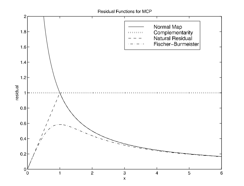
There are several reformulations of the MCP as a system of nonlinear (nonsmooth) equations for which the corresponding residual is a natural merit function. Some of these are as follows:
- Generalized Minimum Map: \(x - \pi(x - F(x))\)
- Normal Map: \(F(\pi(y)) + y - \pi(y)\)
- Fischer Function: \(\Phi(x)\), where \(\Phi_i(x) := \phi(x_i,F_i(x))\) with
\[ \phi(a,b) := \sqrt{a^2 + b^2} - a - b. \]
Note that \(\phi(a,b) = 0\) if and only if \(0 \leq a \perp b \geq 0\). A straightforward extension of \(\Phi\) to the MCP format is given for example in [60] .
In the context of nonlinear complementarity problems the generalized minimum map corresponds to the classic minimum map \(\min(x,F(x))\). Furthermore, for NCPs the minimum map and the Fischer function are both local error bounds and were shown to be equivalent in [185] . Figure 10 in the subsequent section plots all of these merit functions for the ill-defined example discussed therein and highlights the differences between them.
The squared norm of \(\Phi\), namely \(\Psi(x) := \frac{1}{2} \sum \phi(x_i,F_i)^2\), is continuously differentiable on \(\mathbf{R}^n\) provided \(F\) itself is. Therefore, the first order optimality conditions for the unconstrained minimization of \(\Psi(x)\), namely \(\nabla \Psi(x) = 0\) give another indication as to whether the point under consideration is a solution of MCP.
The merit functions and the information PATH provides at the solution can be useful for diagnostic purposes. By default, PATH 4.x returns the best point with respect to the merit function because this iterate likely provides better information to the modeler. As detailed in Section PATH Options, the default merit function in PATH 4.x is the Fischer function. To change this behavior the merit_function option can be used.
Crashing Method
The crashing technique [45] is used to quickly identify an active set from the user-supplied starting point. At this time, a proximal perturbation scheme [23] , [24] is used to overcome problems with a singular basis matrix. The proximal perturbation is introduced in the crash method, when the matrix factored is determined to be singular. The value of the perturbation is based on the current merit function value.
Even if the crash method is turned off, for example via the option crash_method none, perturbation can be added. This is determined by factoring the matrix that crash would have initially formed. This behavior is extremely useful for introducing a perturbation for singular models. It can be turned off by issuing the option crash_perturb no.
Nonmontone Searches
The first line of defense against convergence to stationary points is the use of a nonmonotone linesearch [89] , [90] , [55] . In this case we define a reference value, \(R^k\), and we use this value to test for sufficient decrease:
\[ \Psi (x^k+t_k d^k) \leq \mathbf{R}^k + t_k \nabla \Psi(x^k)^T d^k. \]
Depending upon the choice of the reference value, this allows the merit function to increase from one iteration to the next. This strategy can not only improve convergence, but can also avoid local minimizers by allowing such increases.
We now need to detail our choice of the reference value. We begin by letting \(\{M_1,\ldots,M_m\}\) be a finite set of values initialized to \(\kappa \Psi(x^0)\), where \(\kappa\) is used to determine the initial set of acceptable merit function values. The value of \(\kappa\) defaults to 1 in the code and can be modified with the nms_initial_reference_factor option; \(\kappa=1\) indicates that we are not going to allow the merit function to increase beyond its initial value.
Having defined the values of \(\{M_1,\ldots,M_m\}\) (where the code by default uses \(m=10\)), we can now calculate a reference value. We must be careful when we allow gradient steps in the code. Assuming that \(d^k\) is the Newton direction, we define \(i_0 = \mbox{argmax }M_i\) and \(R^k = M_{i_0}\). After the nonmonotone linesearch rule above finds \(t_k\), we update the memory so that \(M_{i_0} = \Psi(x^k+t_kd^k)\), i.e. we remove an element from the memory having the largest merit function value.
When we decide to use a gradient step, it is beneficial to let \(x^k = x^{\mbox{best}}\) where \(x^{\mbox{best}}\) is the point with the absolute best merit function value encountered so far. We then recalculate \(d^k = -\nabla \Psi(x^k)\) using the best point and let \(R^k = \Psi(x^k)\). That is to say that we force decrease from the best iterate found whenever a gradient step is performed. After a successful step we set \(M_i = \Psi(x^k + t_kd^k)\) for all \(i \in [1, \ldots, m]\). This prevents future iterates from returning to the same problem area.
A watchdog strategy [34] is also available for use in the code.The method employed allows steps to be accepted when they are "close" to the current iterate. Nonmonotonic decrease is enforced every \(m\) iterations, where \(m\) is set by the nms_mstep_frequency option.
Linear Complementarity Problems
PATH solves a linear complementarity problem at each major iteration. Let \(M \in \Re^{n\times n}\), \(q \in \Re^n\), and \(B = [l,u]\) be given. \((\bar{z}, \bar{w}, \bar{v})\) solves the linear mixed complementarity problem defined by \(M\), \(q\), and \(B\) if and only if it satisfies the following constrained system of equations:
\begin{equation} \tag{4} Mz - w + v + q = 0 \label{eq:f1} \end{equation}
\begin{equation} \tag{5} w^T(z - l) = 0 \label{eq:f2} \end{equation}
\begin{equation} \tag{6} v^T(u - z) = 0 \label{eq:f3} \end{equation}
\begin{equation} \tag{7} z \in B, w \in \Re^n_+, v \in \Re^n_+ \end{equation}
where \(x + \infty = \infty\) for all \(x \in \Re\) and \(0\cdot\infty = 0\) by convention. A triple, \((\hat{z}, \hat{w}, \hat{v})\), satisfying equations (4) - (6) is called a complementary triple.
The objective of the linear model solver is to construct a path from a given complementary triple \((\hat{z}, \hat{w}, \hat{v})\) to a solution \((\bar{z}, \bar{w}, \bar{v})\). The algorithm used to solve the linear problem is identical to that given in [47] ; however, artificial variables are incorporated into the model. The augmented system is then:
\begin{equation} \tag{8} Mz - w + v + Da + \frac{(1-t)}{s}(sr) + q = 0 \end{equation}
\begin{equation} \tag{9} w^T(z-l) = 0 \end{equation}
\begin{equation} \tag{10} v^T(u-z) = 0 \end{equation}
\begin{equation} \tag{11} z \in B, w \in \Re^n_+, v \in \Re^n_+, a \equiv 0, t \in [0,1] \end{equation}
where \(r\) is the residual, \(t\) is the path parameter, and \(a\) is a vector of artificial variables. The residual is scaled by \(s\) to improve numerical stability.
The addition of artificial variables enables us to construct an initial invertible basis consistent with the given starting point even under rank deficiency. The procedure consists of two parts: constructing an initial guess as to the basis and then recovering from rank deficiency to obtain an invertible basis. The crash technique gives a good approximation to the active set. The first phase of the algorithm uses this information to construct a basis by partitioning the variables into three sets:
- \(W = \{i \in \{1, \ldots, n\} \mid \hat{z}_i = l_i \mbox{ and } \hat{w}_i > 0\}\)
- \(V = \{i \in \{1, \ldots, n\} \mid \hat{z}_i = u_i \mbox{ and } \hat{v}_i > 0\}\)
- \(Z = \{1, \ldots, n\} \setminus W\cup V\)
Since \((\hat{z}, \hat{w}, \hat{v})\) is a complementary triple, \(Z\cap W\cap V = \emptyset\) and \(Z\cup W\cup V = \{1, \ldots, n\}\). Using the above guess, we can recover an invertible basis consistent with the starting point by defining \(D\) appropriately. The technique relies upon the factorization to indicate the linearly dependent rows and columns of the basis matrix. Some of the variables may be nonbasic, but not at their bounds. For such variables, the corresponding artificial will be basic.
We use a modified version of EXPAND [82] to perform the ratio test. Variables are prioritized as follows:
- \(t\) leaving at its upper bound.
- Any artificial variable.
- Any \(z\), \(w\), or \(v\) variable.
If a choice as to the leaving variable can be made while maintaining numerical stability and sparsity, we choose the variable with the highest priority (lowest number above).
When an artificial variable leaves the basis and a \(z\)-type variable enters, we have the choice of either increasing or decreasing that entering variable because it is nonbasic but not at a bound. The determination is made such that \(t\) increases and stability is preserved.
If the code is forced to use a ray start at each iteration (lemke_start always), then the code carries out Lemke's method, which is known [38] not to cycle. However,by default, we use a regular start to guarantee that the generated path emanates from the current iterate. Under appropriate conditions, this guarantees a decrease in the nonlinear residual. However, it is then possible for the pivot sequence in the linear model to cycle. To prevent this undesirable outcome, we attempt to detect the formation of a cycle with the heuristic that if a variable enters the basis more that a given number of times, we are cycling. The number of times the variable has entered is reset whenever \(t\) increases beyond its previous maximum or an artificial variable leaves the basis. If cycling is detected, we terminate the linear solver at the largest value of \(t\) and return this point.
Another heuristic is added when the linear code terminates on a ray. The returned point in this case is not the base of the ray. We move a slight distance up the ray and return this new point. If we fail to solve the linear subproblem five times in a row, a Lemke ray start will be performed in an attempt to solve the linear subproblem. Computational experience has shown this to be an effective heuristic and generally results in solving the linear model. Using a Lemke ray start is not the default mode, since typically many more pivots are required.
For times when a Lemke start is actually used in the code, an advanced ray can be used. We basically choose the "closest" extreme point of the polytope and choose a ray in the interior of the normal cone at this point. This helps to reduce the number of pivots required. However, this can fail when the basis corresponding to the cell is not invertible. We then revert to the Lemke start.
Since the EXPAND pivot rules are used, some of the variables may be nonbasic, but slightly infeasible, as the solution. Whenever the linear code finishes, the nonbasic variables are put at their bounds and the basic variables are recomputed using the current factorization. This procedure helps to find the best possible solution to the linear system.
The resulting linear solver as modified above is robust and has the desired property that we start from \((\hat{z}, \hat{w}, \hat{v})\) and construct a path to a solution.
Other Features
Some other heuristics are incorporated into the code. During the first iteration, if the linear solver fails to find a Newton point, a Lemke start is used. Furthermore, under repeated failures during the linear solve, a Lemke start will be attempted. A gradient step can also be used when we fail repeatedly.
The proximal perturbation is reduced at each major iteration. However, when numerical difficulties are encountered, it will be increased to a fraction of the current merit function value. These are determined when the linear solver returns a Reset or Singular status.
Spacer steps are taken every major iteration, in which the iterate is chosen to be the best point for the normal map. The corresponding basis passed into the Lemke code is also updated.
Scaling is done based on the diagonal of the matrix passed into the linear solver.
We finally note, that if the merit function fails to show sufficient decrease over the last 100 iterates, a restart will be performed, as this indicates we are close to a stationary point.
Difficult Models
Ill-Defined Models
A problem can be ill-defined for several different reasons. We concentrate on the following particular cases. We will call \(F\) well-defined at \(\bar{x} \in C\) if \(\bar{x} \in D\) and ill-defined at \(\bar{x}\) otherwise. Furthermore, we define \(F\) to be well-defined near \(\bar{x} \in C\) if there exists an open neighborhood of \(\bar{x}\), \(\mathcal{N}(\bar{x})\), such that \(C\cap\mathcal{N}(\bar{x}) \subseteq D\). By saying the function is well-defined near \(\bar{x}\), we are simply stating that \(F\) is defined for all \(x \in C\) sufficiently close to \(\bar{x}\). A function not well-defined near \(\bar{x}\) is termed ill-defined near \(\bar{x}\).
We will say that \(F\) has a well-defined Jacobian at \(\bar{x} \in C\) if there exists an open neighborhood of \(\bar{x}\), \(\mathcal{N}(\bar{x})\), such that \(\mathcal{N}(\bar{x}) \subseteq D\) and \(F\) is continuously differentiable on \(\mathcal{N}(\bar{x})\). Otherwise the function has an ill-defined Jacobian at \(\bar{x}\). We note that a well-defined Jacobian at \(\bar{x}\) implies that the MCP has a well-defined function near \(\bar{x}\), but the converse is not true.
PATH uses both function and Jacobian information in its attempt to solve the MCP. Therefore, both of these definitions are relevant. We discuss cases where the function and Jacobian are ill-defined in the next two subsections. We illustrate uses for the merit function information and final point statistics within the context of these problems.
Function Undefined We begin with a one-dimensional problem for which \(F\) is ill-defined at \(x = 0\) as follows:
\[ \begin{array}{rcl} 0 \leq x & \perp & \frac{1}{x} \geq 0. \end{array} \]
Here \(x\) must be strictly positive because \(\frac{1}{x}\) is undefined at \(x = 0\). This condition implies that \(F(x)\) must be equal to zero. Since \(F(x)\) is strictly positive for all \(x\) strictly positive, this problem has no solution.
We are able to perform this analysis because the dimension of the problem is small. Preprocessing linear problems can be done by the solver in an attempt to detect obviously inconsistent problems, reduce problem size, and identify active components at the solution. Similar processing can be done for nonlinear models, but the analysis becomes more difficult to perform. Currently, PATH only checks the consistency of the bounds and removes fixed variables and the corresponding complementary equations from the model.
A modeler would likely not know a priori that a problem has no solution and would thus attempt to formulate and solve it. GAMS code for the model above is provided in Figure 8. We must specify an initial value for \(x\) in the code. If we were to not provide one, GAMS would use \(x = 0\) as the default value, notice that \(F\) is undefined at the initial point, and terminate before giving the problem to PATH. The error message indicates that the function \(\frac{1}{x}\) is ill-defined at \(x = 0\), but does not imply that the corresponding MCP problem has no solution.
Figure 8: GAMS Code for Ill-Defined Function
positive variable x;
equations F;

F.. 1 / x =g= 0;

model simple / F.x /;

x.l = 1e-6;

solve simple using mcp;
After setting the starting point, GAMS generates the model, and PATH proceeds to "solve" it. A portion of the output relating statistics about the solution is given in Figure 9 PATH uses the Fischer Function indicator as its termination criteria by default, but evaluates all of the merit functions given in Section Merit Functions at the final point. The Normal Map merit function, and to a lesser extent, the complementarity error, indicate that the "solution" found does not necessarily solve the MCP.
Figure 9: PATH Output for Ill-Defined Function
FINAL STATISTICS
Inf-Norm of Complementarity . .  1.0000e+00 eqn: (F)
Inf-Norm of Normal Map. . . . .  1.1181e+16 eqn: (F)
Inf-Norm of Minimum Map . . . .  8.9441e-17 eqn: (F)
Inf-Norm of Fischer Function. .  8.9441e-17 eqn: (F)
Inf-Norm of Grad Fischer Fcn. .  8.9441e-17 eqn: (F)

FINAL POINT STATISTICS
Maximum of X. . . . . . . . . .  8.9441e-17 var: (X)
Maximum of F. . . . . . . . . .  1.1181e+16 eqn: (F)
Maximum of Grad F . . . . . . .  1.2501e+32 eqn: (F)
                                            var: (X)
To indicate the difference between the merit functions, Figure 10 plots them all for this simple example. We note that as \(x\) approaches positive infinity, numerically, we are at a solution to the problem with respect to all of the merit functions except for the complementarity error, which remains equal to one. As \(x\) approaches zero, the merit functions diverge, also indicating that \(x = 0\) is not a solution.
The natural residual and Fischer function tend toward \(0\) as \(x \downarrow 0\). From these measures, we might think \(x = 0\) is the solution. However, as previously remarked \(F\) is ill-defined at \(x = 0\). \(F\) and \(\nabla F\) become very large, indicating that the function (and Jacobian) might not be well-defined. We might be tempted to conclude that if one of the merit function indicators is not close to zero, then we have not found a solution. This conclusion is not always warranted. When one of the indicators is non-zero, we have reservations about the solution, but we cannot eliminate the possibility that we are actually close to a solution. If we slightly perturb the original problem to
\[ \begin{array}{rcl} 0 \leq x & \perp & \frac{1}{x + \epsilon} \geq 0 \end{array} \]
for a fixed \(\epsilon > 0\), the function is well-defined over \(C = \mathbf{R}^n_+\) and has a unique solution at \(x = 0\). In this case, by starting at \(x > 0\) and sufficiently small, all of the merit functions, with the exception of the Normal Map, indicate that we have solved the problem as is shown by the output in Figure 11 for \(\epsilon = 1*10^{-6}\) and \(x = 1*10^{-20}\).
Figure 11: PATH Output for Well-Defined Function
FINAL STATISTICS
Inf-Norm of Complementarity . .  1.0000e-14 eqn: (G)
Inf-Norm of Normal Map. . . . .  1.0000e+06 eqn: (G)
Inf-Norm of Minimum Map . . . .  1.0000e-20 eqn: (G)
Inf-Norm of Fischer Function. .  1.0000e-20 eqn: (G)
Inf-Norm of Grad Fischer Fcn. .  1.0000e-20 eqn: (G)

FINAL POINT STATISTICS
Maximum of X. . . . . . . . . .  1.0000e-20 var: (X)
Maximum of F. . . . . . . . . .  1.0000e+06 eqn: (G)
Maximum of Grad F . . . . . . .  1.0000e+12 eqn: (G)
                                            var: (X)
In this case, the Normal Map is quite large and we might think that the function and Jacobian are undefined. When only the normal map is non-zero, we may have just mis-identified the optimal basis. By setting the merit_function normal option, we can resolve the problem, identify the correct basis, and solve the problem with all indicators being close to zero. This example illustrates the point that all of these tests are not infallible. The modeler still needs to do some detective work to determine if they have found a solution or if the algorithm is converging to a point where the function is ill-defined.
Jacobian Undefined Since PATH uses a Newton-like method to solve the problem, it also needs the Jacobian of \(F\) to be well-defined. One model for which the function is well-defined over \(C\), but for which the Jacobian is undefined at the solution is: \(0 \le x \perp -\sqrt{x} \ge 0\). This model has a unique solution at \(x = 0\).
Using PATH and starting from the point \(x = 1*10^{-14}\), PATH generates the output given in Figure 12 .
Figure 12: PATH Output for Ill-Defined Jacobian
FINAL STATISTICS
Inf-Norm of Complementarity . .  1.0000e-07 eqn: (F)
Inf-Norm of Normal Map. . . . .  1.0000e-07 eqn: (F)
Inf-Norm of Minimum Map . . . .  1.0000e-07 eqn: (F)
Inf-Norm of Fischer Function. .  2.0000e-07 eqn: (F)
Inf-Norm of Grad FB Function. .  2.0000e+00 eqn: (F)

FINAL POINT STATISTICS
Maximum of X. . . . . . . . . .  1.0000e-14 var: (X)
Maximum of F. . . . . . . . . .  1.0000e-07 eqn: (F)
Maximum of Grad F . . . . . . .  5.0000e+06 eqn: (F)
                                            var: (X)
We can see that the gradient of the Fischer Function is nonzero and the Jacobian is beginning to become large. These conditions indicate that the Jacobian is undefined at the solution. It is therefore important for a modeler to inspect the given output to guard against such problems.
If we start from \(x = 0\), PATH correctly informs us that we are at the solution. The large value reported for the Jacobian is an indication that the Jacobian is undefined.
Poorly Scaled Models
Well-defined problems can still have various numerical problems that impede the algorithm's convergence. One particular problem is a badly scaled Jacobian. In such cases, we can obtain a poor "Newton" direction because of numerical problems introduced in the linear algebra performed. This problem can also lead the code to a point from which it cannot recover.
The final model given to the solver should be scaled such that we avoid numerical difficulties in the linear algebra. The output provided by PATH can be used to iteratively refine the model so that we eventually end up with a well-scaled problem. We note that we only calculate our scaling statistics at the starting point provided. For nonlinear problems these statistics may not be indicative of the overall scaling of the model. Model specific knowledge is very important when we have a nonlinear problem because it can be used to appropriately scale the model to achieve a desired result.
We look at the titan.gms model in MCPLIB, that has some scaling problems. The relevant output from PATH for the original code is given in Figure 13.
Figure 13: PATH Output - Poorly Scaled Model
INITIAL POINT STATISTICS
Maximum of X. . . . . . . . . .  4.1279e+06 var: (w.29)
Maximum of F. . . . . . . . . .  2.2516e+00 eqn: (a1.33)
Maximum of Grad F . . . . . . .  6.7753e+06 eqn: (a1.29)
                                            var: (x1.29)

INITIAL JACOBIAN NORM STATISTICS
Maximum Row Norm. . . . . . . .  9.4504e+06 eqn: (a2.29)
Minimum Row Norm. . . . . . . .  2.7680e-03 eqn: (g.10)
Maximum Column Norm . . . . . .  9.4504e+06 var: (x2.29)
Minimum Column Norm . . . . . .  1.3840e-03 var: (w.10)
The maximum row norm is defined as
\[ \max_{1 \le i \le n} \sum_{1 \le j \le n} \mid (\nabla F(x))_{ij} \mid \]
and the minimum row norm is
\[ \min_{1 \le i \le n} \sum_{1 \le j \le n} \mid (\nabla F(x))_{ij} \mid . \]
Similar definitions are used for the column norm. The norm numbers for this particular example are not extremely large, but we can nevertheless improve the scaling. We first decided to reduce the magnitude of the a1 block of equations as indicated by PATH. Using the GAMS modeling language, we can scale particular equations and variables using the .scale attribute. To turn the scaling on for the model we use the .scaleopt model attribute. After scaling the a1 block, we re-ran PATH and found an additional block of equations that also needed scaling, a2. We also scaled some of the variables, g and w. The code added to the model follows:
     titan.scaleopt = 1;
     a1.scale(i) = 1000;
     a2.scale(i) = 1000;
     g.scale(i) = 1/1000;
     w.scale(i) = 100000;
By scaling these equation and variable blocks, we have improved the model scaling. The statistics for the manually scaled model are given in Figure 14.
Figure 14: PATH Output - Well-Scaled Model
INITIAL POINT STATISTICS
Maximum of X. . . . . . . . . .  1.0750e+03 var: (x1.49)
Maximum of F. . . . . . . . . .  3.9829e-01 eqn: (g.10)
Maximum of Grad F . . . . . . .  6.7753e+03 eqn: (a1.29)
                                            var: (x1.29)

INITIAL JACOBIAN NORM STATISTICS
Maximum Row Norm. . . . . . . .  9.4524e+03 eqn: (a2.29)
Minimum Row Norm. . . . . . . .  2.7680e+00 eqn: (g.10)
Maximum Column Norm . . . . . .  9.4904e+03 var: (x2.29)
Minimum Column Norm . . . . . .  1.3840e-01 var: (w.10)
For this particular problem PATH cannot solve the unscaled model, while it can find a solution to the scaled model. Using the scaling features of the GAMS language and the information provided by PATH we are able to remove some of the problem's difficulty and obtain better performance from PATH.
It is possible to get even more information on initial point scaling by inspecting the GAMS listing file. The equation row listing gives the values of all the entries of the Jacobian at the starting point. The row norms generated by PATH give good pointers for starting to use the row listing.
Not all of the numerical problems are directly attributable to poorly scaled models. Problems for which the Jacobian of the active constraints is singular or nearly singular can also cause numerical difficulty as illustrated next.
Singular Models
Assuming that the problem is well-defined and properly scaled, we can still have a Jacobian for which the active constraints are singular or nearly singular (i.e. it is ill-conditioned). When problems are singular or nearly singular, we are also likely to have numerical problems. As a result the "Newton" direction obtained from the linear problem solver can be very bad. In PATH, we can use proximal perturbation or add artificial variables to attempt to remove the singularity problems from the model. However, it is most often beneficial for solver robustness to remove singularities if possible.
The easiest problems to detect are those for which the Jacobian has zero rows and columns. A simple problem for which we have zero rows and columns is:
\[ \begin{array}{rcl} -2 \leq x \leq 2 & \perp & -x^2 + 1. \end{array} \]
Note that the Jacobian, \(-2x\), is non-singular at all three solutions, but singular at the point \(x = 0\). Output from PATH on this model starting at \(x = 0\) is given in Figure 15.
Figure 15: PATH Output - Zero Rows and Columns
INITIAL POINT STATISTICS
Zero column of order. . . . . .  0.0000e+00 var: (X)
Zero row of order . . . . . . .  0.0000e+00 eqn: (F)
Total zero columns. . . . . . .  1
Total zero rows . . . . . . . .  1
Maximum of F. . . . . . . . . .  1.0000e+00 eqn: (F)
Maximum of Grad F . . . . . . .  0.0000e+00 eqn: (F)
                                            var: (X)
We display in the code the variables and equations for which the row/column in the Jacobian is close to zero. These situations are problematic and for nonlinear problems likely stem from the modeler providing an inappropriate starting point or fixing some variables resulting in some equations becoming constant. We note that the solver may perform well in the presence of zero rows and/or columns, but the modeler should make sure that these are what was intended.
Singularities in the model can also be detected by the linear solver. This in itself is a hard problem and prone to error. For matrices which are poorly scaled, we can incorrectly identify "linearly dependent" rows because of numerical problems. Setting output_factorization_singularities yes in an options file will inform the user which equations the linear solver thinks are linearly dependent. Typically, singularity does not cause a lot of problems and the algorithm can handle the situation appropriately. However, an excessive number of singularities are cause for concern. A further indication of possible singularities at the solution is a lack of quadratic convergence to the solution.
Case Study: Von Thunen Land Model
We now turn our attention towards using the diagnostic information provided by PATH to improve an actual model. The Von Thunen land model is a problem recognized in the mathematical programming literature for its computational difficulty. We attempt to understand more carefully the facets of the problem that make it difficult to solve. This will enable us to outline and identify these problems and furthermore to extend the model to a more realistic and computationally more tractable form.
Classical Model
The problem is cast in the Arrow-Debreu framework as an equilibrium problem.The basic model is a closed economy consisting of three economic agents, a landowner, a worker and a porter. There is a central market, around which concentric regions of land are located. Since the produced goods have to be delivered to the market, this is an example of a spatial price equilibrium. The key variables of the model are the prices of commodities, land, labour and transport. Given these prices, it is assumed that the agents demand certain amounts of the commodities, which are supplied so as to maximize profit in each sector. Walras' law is then a consequence of the assumed competitive paradigm, namely that supply will equal demand in the equilibrium state.
We now describe the problems that the consumers and the producers face. We first look at consumption and derive a demand function for each of the consumer agents in the economy. Each of these agents has a utility function, that they wish to maximize subject to their budgetary constraints. As is typical in such problems, the utility function is assumed to be Cobb-Douglas:
\[ u_a(d) = \prod_{c} d_c^{\alpha_{c,a}}, \quad \alpha_{c,a} \geq 0, \sum_{c} \alpha_{c,a} = 1, \]
where the \(\alpha_{c,a}\) are given parameters dependent only on the agent. For each agent \(a\), the variables \(d_{c}\) represent quantities of the desired commodities \(c\). In the Von Thunen model, the goods are wheat, rice, corn and barley. The agent's endowments determine their budgetary constraint as follows. Given current market prices, an agent's wealth is the value of the initial endowment of goods at those prices. The agent's problem is therefore
\[ \max_d u_a(d) \text{ subject to } \langle p,d \rangle \leq \langle p,{e_a}\rangle, d \geq 0 , \]
where \(e_a\) is the endowment bundle for agent a. A closed form solution, corresponding to demand from agent \(a\) for commodity \(c\) is thus
\[ d_{c,a}(p) := \frac{\alpha_{c,a} \langle p,e_a \rangle }{p_c} . \]
Note that this assumes the prices of the commodities \(p_c\) are positive.
The supply side of the economy is similar. The worker earns a wage \(w_L\) for his labour input. The land is distributed around the market in rings with a rental rate \(w_r\) associated with each ring \(r\) of land. The area of land \(a_r\) in each ring is an increasing function of \(r\). The model assumes that labour and land are substitutable via a constant elasticities of substitution (CES) function.
Consider the production \(x_{c,r}\) of commodity \(c\) in region \(r\). In order to maximize profit (or minimize costs), the labour \(y_L\) and land use \(y_r\) solve
\begin{equation} \tag{12} \min w_L y_L + w_r y_r \text{ subject to } \phi_c y_L^{\beta_c} y_r^{1 - \beta_c} \geq x_{c,r},\; y_L, y_r \geq 0 , \end{equation}
where \(\phi_c\) is a given cost function scale parameter, and \(\beta_c \in [0,1]\) is the share parameter. The technology constraint is precisely the CES function allowing a suitable mix of labour and land use. Again, a closed form solution can be calculated. For example, the demand for labour in order to produce \(x_{c,r}\) of commodity \(c\) in region \(r\) is given by
\[ x_{c,r} \frac{\beta_c \left(\frac{w_L}{\beta_c}\right)^{\beta_c} \left(\frac{w_r}{1-\beta_c}\right)^{1-\beta_c}}{\phi_c w_L} . \]
Considering all such demands, this clearly assumes the prices of inputs \(w_L\), \(w_r\) are positive. A key point to note is that input commodity (factor) demands to produce \(x_{c,r}\) can be determined by first solving (12) for unit demand \(x_{c,r} \equiv 1\) and then multiplying these factor demands by the actual amount desired. Let \(\bar{y}_L\) and \(\bar{y}_r\) denote the optimal solutions of (12) with \(x_{c,r} \equiv 1\). Using this fact, the unit production cost \(\gamma_{c,r}\) for commodity \(c\) in region \(r\) can be calculated as follows:
\begin{eqnarray*} \gamma_{c,r} & = & w_L \bar{y}_L + w_r \bar{y}_r \\ & = & w_L \frac{\beta_c \left(\frac{w_L}{\beta_c}\right)^{\beta_c} \left(\frac{w_r}{1-\beta_c}\right)^{1-\beta_c}}{\phi_c w_L} + w_r \frac{(1-\beta_c) \left(\frac{w_L}{\beta_c}\right)^{\beta_c} \left(\frac{w_r}{1-\beta_c}\right)^{1-\beta_c}}{\phi_c w_r} \\ & = & \frac{1}{\phi_c}\left(\frac{w_L}{\beta_c}\right)^{\beta_c} \left(\frac{w_r}{1-\beta_c}\right)^{1-\beta_c} . \end{eqnarray*}
Transportation is provided by a porter, earning a wage \(w_p\). If we denote the unit cost for transportation of commodity \(c\) by \(t_c\), then unit transportation cost to market is
\[ T_{c,r}(w_p) := t_c d_r w_p , \]
where \(d_r\) is the distance of region \(r\) to the market. Spatial price equilibrium arises from the consideration:
\[ 0 \leq x_{c,r} \perp \gamma_{c,r}(w_L,w_r) + T_{c,r}(w_p) \geq p_c . \]
This is intuitively clear; it states that commodity \(c\) will be produced in region \(r\) only if the combined cost of production and transportation equals the market price.
The above derivations assumed that the producers and consumers acted as price takers. Walras' law is now invoked to determine the prices so that markets clear. The resulting complementarity problem is:
\begin{equation} \tag{13} \gamma_{c,r} = \frac{1}{\phi_c}\left(\frac{w_L}{\beta_c}\right)^{\beta_c} \left(\frac{w_r}{1-\beta_c}\right)^{1-\beta_c} \end{equation}
\begin{equation} \tag{14} 0 \leq x_{c,r} \perp \gamma_{c,r} + T_{c,r}(w_p) \geq p_c \end{equation}
\begin{equation} \tag{15} 0 \leq w_L \perp e_L \geq \sum_{r,c} x_{c,r} \frac{\beta_c \gamma_{c,r} }{ w_L} \end{equation}
\begin{equation} \tag{16} 0 \leq w_r \perp a_r \geq \sum_c \frac{x_{c,r} (1-\beta_c) \gamma_{c,r}}{ w_r } \end{equation}
\begin{equation} \tag{17} 0 \leq w_p \perp e_P \geq \sum_{r,c} t_c d_r x_{c,r} \end{equation}
\begin{equation} \tag{18} 0 \leq p_c \perp \sum_r x_{c,r} \geq \frac{\alpha_{c,P} e_P w_p + \alpha_{c,L} e_L w_L + \alpha_{c,O} \sum_r w_r a_r}{p_c} \end{equation}
Note that in (15), (16) and (17), the amounts of labour, land and transport are bounded from above, and hence the prices on these inputs are determined as multipliers (or shadow prices) on the corresponding constraints. The final relationship (18) in the above complementarity problem corresponds to market clearance; prices are nonnegative and can only be positive if supply equals demand. (Some modelers multiply the last inequality throughout by \(p_c\). This removes problems where \(p_c\) becomes zero, but can also introduce spurious solutions.)
The Arrow-Debreu theory guarantees that the problem is homogeneous in prices; \((x,\lambda w,\lambda p)\) is also a solution whenever \((x,w,p)\) solves the above. Typically this singularity in the model is removed by fixing a numeraire, that is fixing a price (for example \(w_L = 1\)) and dropping the corresponding complementary relationship.
Unfortunately, in this formulation even after fixing a numeraire, some of the variables \(p\) and \(w\) may go to zero, resulting in an ill-defined problem. In the case of the Von Thunen land model, the rental price of land \(w_r\) decreases as the distance to market increases, and for remote rings of land, it becomes zero. A standard modeling fix is to put artificial lower bounds on these variables. Even with this fix, the problem typically remains very hard to solve. More importantly, the homogeneity property of the prices used above to fix a numeraire no longer holds, and the corresponding complementary relationship (which was dropped from the problem) may fail to be satisfied. It therefore matters which numeriare is fixed, and many modelers run into difficulty since in many cases the solution found by a solver is invalid for the originally posed model.
In order to test our diagnostic information, we implemented a version of the above model in GAMS. The model corresponds closely to the MCPLIB model pgvon105.gms except we added more regions to make the problem even more difficult. The model file has been documented more fully, and the data rounded to improve clarity.
Our first trial was to solve the model without fixing a numeraire. In this case, PATH 4.x failed to find a solution. At the starting point, the indicators described in Sectiion Ill-Defined Models are reasonable, and there are no zero rows/columns in the Jacobian. At the best point found, all indicators are still reasonable. However, the listing file indicates a large number of division by zero problems occurring in (16). We also note that a nonzero proximal perturbation is used in the first iteration of the crash method. This is an indication of singularities. We therefore added an option to output factorization singularities, and singularities appeared in the first iteration. At this point, we decided to fix a numeraire to see if this alleviated the problem.
We chose to fix the labour wage rate to 1. After increasing the iterations allowed to 100,000, PATH 4.x solved the problem. The statistics at the solution are cause for concern. In particular, the gradient of the Fischer function is 7 orders of magnitude larger than all the other residuals. Furthermore, the Jacobian is very large at the solution point. Looking further in the listing file, a large number of division by zero problems occur in (16).
To track down the problem further, we added an artificial lower bound on the variables \(w_r\) of \(10^{-5}\), that would not be active at the aforementioned solution. Resolving gave the same "solution", but resulted in the domain errors disappearing.
Although the problem is solved, there is concern on two fronts. Firstly, the gradient of the Fischer function should go to zero at the solution. Secondly, if a modeler happens to make the artificial lower bounds on the variables a bit larger, then they become active at the solution, and hence the constraint that has been dropped by fixing the price of labour at 1 is violated at this point. Of course, the algorithm is unable to detect this problem, since it is not part of the model that is passed to it, and the corresponding output looks satisfactory.
We are therefore led to the conclusion that the model as postulated is ill-defined. The remainder of this section outlines two possible modeling techniques to overcome the difficulties with ill-defined problems of this type.
Intervention Pricing
The principal difficulty is the fact that the rental prices on land go to zero as proximity to the market decreases, and become zero for sufficiently remote rings. Such a property is unlikely to hold in a practical setting. Typically, a landowner has a minimum rental price (for example, land in fallow increases in value). As outlined above, a fixed lower bound on the rental price violates the well-established homogeneity property. A suggestion postulated by Professor Thomas Rutherford is to allow the landowner to intervene and "purchase-back" his land whenever the rental cost gets smaller than a certain fraction of the labour wage.
The new model adds a (homogeneous in price) constraint
\[ \begin{array}{lcr} 0 \leq i_r & \perp & w_r \geq 0.0001 * w_L \end{array} \]
and modifies (16) and (18) as follows:
\begin{equation*} 0 \leq w_r \perp a_r - i_r \geq \sum_c \frac{x_{c,r} (1-\beta_c) \gamma_{c,r}}{ w_r } \end{equation*}
\begin{equation} \tag{19} 0 \leq p_c \perp \sum_r x_{c,r} \geq \frac{\alpha_{c,P} e_P w_p + \alpha_{c,L} e_L w_L + \alpha_{c,O} \sum_r w_r (a_r - i_r)}{p_c}. \end{equation}
Given the intervention purchase, we can now add a lower bound on \(w_r\) to avoid division by zero errors. In our model we chose \(10^{-5}\) since this will never be active at the solution and therefore will not affect the positive homogeneity. After this reformulation, PATH 4.x solves the problem. Furthermore, the gradient of the Fischer function, although slightly larger than the other residuals, is quite small, and can be made even smaller by reducing the convergence tolerance of PATH. Inspecting the listing file, the only difficulties mentioned are division by zero errors in the market clearance condition (19), that can be avoided a posteori by imposing an artificial (inactive) lower bound on these prices. We chose not to do this however.
Nested Production and Maintenance
Another observation that can be used to overcome the land price going to zero is the fact that land typically requires some maintenance labour input to keep it usable for crop growth. Traditionally, in economics, this is carried out by providing a nested CES function as technology input to the model. The idea is that commodity \(c\) in region \(r\) is made from labour and an intermediate good, which is "maintained land". Essentially, the following production problem replaces (12):
\[ \begin{array}{rc} \min_{y_M,y_L,y_r,g} & w_L (y_M + y_L) + w_r y_r \\ \text{ subject to } & y_r \geq (1 - \beta_c - \epsilon) g \\ & y_M \geq \epsilon g \\ & \phi_c y_L^{\beta_c} g^{1 - \beta_c} \geq 1,\\ & y_M, y_L, y_r, g \geq 0 . \end{array} \]
Note that the variable \(y_M\) represents "maintenance labour" and \(g\) represents the amount of "maintained land" produced, an intermediate good. The process of generating maintained land uses a Leontieff production function, namely
\[ \min ( \lambda_r y_r, \lambda_M y_M ) \geq g . \]
Here \(\lambda_M = \frac{1}{\epsilon}\), \(\epsilon\) small, corresponds to small amounts of maintenance labour, while \(\lambda_r =\frac{1}{1-\beta_c-\epsilon}\) is chosen to calibrate the model correctly. A simple calculus exercise then generates appropriate demand and cost expressions. The resulting complementarity problem comprises (14), (17), (18) and
\begin{eqnarray*} & & \gamma_{c,r} = \frac{w_L^{\beta_c}}{\phi_c} \left(\frac{w_L\epsilon + w_r(1-\beta_c-\epsilon)}{1-\beta_c}\right)^{1-\beta_c} \\ 0 \leq w_L & \perp & e_L \geq \sum_{r,c} x_{c,r} \gamma_{c,r} \left(\frac{\beta_c}{w_L} + \frac{\epsilon (1 - \beta_c)}{w_L\epsilon + w_r(1-\beta_c-\epsilon)}\right) \\ 0 \leq w_r & \perp & a_r \geq \sum_c \frac{x_{c,r} \gamma_{c,r} (1-\beta_c) (1-\beta_c - \epsilon) }{w_L\epsilon + w_r(1-\beta_c-\epsilon)} \end{eqnarray*}
After making the appropriate modifications to the model file, PATH 4.x solved the problem on defaults without any difficulties. All indicators showed the problem and solution found to be well-posed.