Table of Contents
- The Basics
- The Calibrated Share Form
- Exercises
- Flexibility and Non-Separable CES functions
- Two NNCES calibrations for a 3-input cost functions
- A Comparison of Locally-Identical Functions
- Numerical calibration of NNCES given KLEM elasticities
- Calibrating Labor Supply and Savings Demand
- A Maquette Illustrating Labor Supply and Savings Demand Calibration
Notes prepared for GAMS General Equilibrium Workshop held December, 1995 in Boulder Colorado.
- Date
- December, 1995
The Basics
In many economic textbooks the constant elasticity of substitution (CES) utility function is defined as:
\[ U(x,y)=(\alpha x^\rho+(1-\alpha)y^\rho)^{\frac{1}{\rho}} , \]
It is a fairly routine but tedious calculus exercise to demonstrate that the associated demand functions are:
\[ x(p_x,p_y,M)=\bigg( \frac{\alpha}{p_x}\bigg)^\sigma =\frac{M}{\alpha^\sigma p^{1-\sigma}_x+(1-\alpha)^\sigma p^{1-\sigma}_{y}} , \]
and
\[ y(p_x,p_y,M)=\bigg( \frac{1-\alpha}{p_y}\bigg)^\sigma \frac{M}{\alpha^\sigma p^{1-\sigma}_x+(1-\alpha)^\sigma p^{1-\sigma}_{y}} , \]
The corresponding indirect utility function has is:
\[ V(p_x,p_y,M)= M \bigg(\alpha^\sigma p^{1-\sigma}_x+(1-\alpha)^\sigma p^{1-\sigma}_{y}\bigg)^{\frac{1}{\sigma -1}} , \]
Note that U(x,y) is linearly homogeneous:
\[ U(\lambda_x,\lambda_y)=\lambda U(x,y) \]
This is a convenient cardinalization of utility, because percentage changes in \(U\) are equivalent to percentage Hicksian equivalent variations in income.
Because \(U\) is linearly homogeneous, \(V\) is homogeneous of degree one in M and degree \(-1\) in \(p\).
In the representation of technology, we have an analogous set of relationships, based on the cost and compensated demand functions. If we have a CES production function of the form:
\[ y(K,L)=\gamma\big( \alpha K^\rho+ (1-\alpha)L^\rho \big)^{\frac{1}{\rho}}, \]
the unit cost function then has the form:
\[ c(p_K,p_L)=\big(\frac {1}{\gamma}\big) \bigg(\alpha^\sigma p^{1-\sigma}_K+ (1-\alpha)^\sigma p^{1-\sigma}_L \bigg)^{\frac{1}{1-\sigma}}, \]
and associated demand functions are:
\[ K(p_K,p_L)=\bigg( \frac {y}{\gamma} \bigg) \bigg(\frac{\alpha\gamma c (p_K,p_L)}{p_K}\bigg)^\sigma , \]
and
\[ L(p_K,p_L)=\bigg( \frac {y}{\gamma} \bigg) \bigg(\frac{(1-\alpha)\gamma c (p_K,p_L)}{p_L}\bigg)^\sigma . \]
In most large-scale applied general equilibrium models, we have many function parameters to specify with relatively few observations. The conventional approach is to calibrate functional parameters to a single benchmark equilibrium. For example, if we have benchmark estimates for output, labor, capital inputs and factor prices , we calibrate function coefficients by inverting the factor demand functions:
\[ \begin{array}{rcll} \theta =\frac{\bar{p}_k \bar{K}}{\bar{p}_k \bar{K}+\bar{P}_L \bar{L}}, & \rho=\frac{\sigma-1}{\sigma}, & \alpha=\theta \bar{K}^{\frac{-1}{\rho}} , \end{array} \]
and
\[ \gamma = \bar{y}\big[ \alpha \bar{K}^\rho + (1-\alpha)\bar{L}^\rho \big]^{\frac{-1}{\rho}}. \]
The Calibrated Share Form
Calibration formulae for CES functions are messy and difficult to remember. Consequently, the specification of function coefficients is complicated and error-prone. For applied work using calibrated functions, it is much easier to use the "calibrated share form" of the CES function. In the calibrated form, the cost and demand functions explicitly incorporate
- benchmark factor demands
- benchmark factor prices
- the elasticity of substitution
- benchmark cost
- benchmark output
- benchmark value shares
In this form, the production function is written:
\[ y=\bar{y} \bigg [ \theta \bigg( \frac{K}{\bar{K}}\bigg)^\rho + (1-\theta)\bigg( \frac{L}{\bar{L}} \bigg)^\rho \bigg ]^{\frac{1}{\rho}} \]
The only calibrated parameter, \(\theta\) , represents the value share of capital at the benchmark point. The corresponding cost functions in the calibrated form is written:
\[ c(p_K,p_L)=\bar{c} \bigg [ \theta \bigg( \frac{p_K}{\bar{p}_k}\bigg)^{1-\sigma} + (1-\theta)\bigg( \frac{p_L}{\bar{p}_L} \bigg)^{1-\sigma} \bigg ]^{\frac{1}{1-\sigma}} \]
where \(\bar{c}=\bar{p}_L \bar{L}+\bar{p}_K \bar{K}\)and the compensated demand functions are:
\[ K(p_K,p_L,y)=\bar{K} \frac{y}{\bar{y}}\bigg ( \frac{\bar{p}_K~c}{p_K~\bar{c}} \bigg )^\sigma \]
and
\[ L(p_K,p_L,y)=\bar{L} \frac{y}{\bar{y}}\bigg ( \frac{c~\bar{p}_L}{\bar{c}~p_K} \bigg )^\sigma . \]
Normalizing the benchmark utility index to unity, the utility function in calibrated share form is written:
\[ U(x,y)=\bigg [ \theta \bigg( \frac{x}{\bar{x}} \bigg )^\rho + (1-\theta) \bigg (\frac{y}{\bar{y}}^\rho \bigg ) \bigg ]^{\frac{1}{\rho}} \]
Defining the unit expenditure function as:
\[ e(p_x,p_y)=\bigg [ \theta \bigg( \frac{p_x}{\bar{p}_x} \bigg )^{1-\sigma} + (1-\theta) \bigg (\frac{p_y}{\bar{p}_y} \bigg ) \bigg ]^{\frac{1}{1-\sigma}} \]
the indirect utility function is:
\[ V(p_x,p_y,M)= \frac{M}{\bar{M}e(p_x,p_y)} \]
and the demand functions are:
\[ x(p_x,p_y,M)=\bar{x}~V(p_x,p_y,M)\bigg ( \frac{e(p_x,p_y)\bar{p}_x}{p_x}\bigg )^\sigma \]
and
\[ y(p_x,p_y,M)=\bar{y}~ V(p_x,p_y,M)\bigg ( \frac{e(p_x,p_y)\bar{p}_y}{p_y}\bigg )^\sigma \]
The calibrated form extends directly to the n-factor case. An n-factor production function is written:
\[ y=f(x)=\bar{y} \bigg [ \sum_i \theta_i \bigg ( \frac {x_i} {\bar{x}_i}\bigg )^\rho \bigg ]^{\frac {1}{\rho}} \]
and has unit cost function:
\[ C(p)=\bar{C} \bigg [ \sum_i \theta_i \bigg ( \frac {p_i} {\bar{p}_i}\bigg )^{1-\sigma} \bigg ]^{\frac {1}{1-\sigma}} \]
and compensated factor demands:
\[ x_i=\bar{x}_i \frac {y}{\bar{y}} \bigg ( \frac {C \bar{p}_i} {\bar{C}p_i}\bigg )^\sigma \]
Exercises
(i) Show that given a generic CES utility function:
\[ U(x,y)=(\alpha^\rho + (1-\alpha) y ^\rho)^ \frac{1}{p} \]
can be represented in share form using:
\[ \bar{x}=1,~ \bar{y}=1,~ \bar{p}_x=t\alpha, ~~ \bar{p}_y=t(1-\alpha), ~\bar{M}=t . \]
for any value of \(t > 0\).
(ii) Consider the utility function defined:
\[ U(x,y)=(x-a)^\alpha (y-b)^{1-\alpha} \]
A benchmark demand point with both prices equal and demand for y equal to twice the demand for \(x\). Find values for which are consistent with optimal choice at the benchmark. Select these parameters so that the income elasticity of demand for \(x\) at the benchmark point equals 1.1.
(iii) Consider the utility function:
\[ U(x,L)=(\alpha L^\rho+(1-\alpha)x^\rho)^\frac{1}{\rho} \]
which is maximized subject to the budget constraint:
\[ p_x x= M+ \omega (\bar{L}-L) \]
in which \(M\) is interpreted as non-wage income, \(\omega\) is the market wage rate. Assume a benchmark equilibrium in which prices for \(x\) and \(L\) are equal, demands for \(x\) and \(L\) are equal, and non-wage income equals one-half of expenditure on \(x\). Find values of \(\alpha\) and \(\rho\) consistent with these choices and for which the price elasticity of labor supply equals 0.2.
(iv) Consider a consumer with CES preferences over two goods. A price change makes the benchmark consumption bundle unaffordable, yet the consumer is indifferent. Graph the choice. Find an equation which determines the elasticity of substitution as a function of the benchmark value shares. (You can write down the equation, but it cannot be solved in closed form.)
(v) Consider a model with three commodities, \(x\), \(y\), and \(z\). Preferences are CES. Benchmark demands and prices are equal for all goods. Find demands for \(x\), \(y\) and \(z\) for a doubling in the price of \(x\) as a function of the elasticity of substitution.
(iv) Consider the same model in the immediately preceeding question, except assume that preferences are instead given by:
\[ U(x,y,z)=(\beta \textrm{min} (x,y)^\rho + (1-\beta) z^\rho)^\frac{1}{\rho} \]
Determine \(\beta\)from the benchmark, and find demands for \(x\), \(y\) and \(z\) if the price of \(x\) doubles.
Flexibility and Non-Separable CES functions
We let \(\pi_i\) denote the user price of the ith input, and let \(x_i(\pi)\) be the cost-minizing demand for the ith input. The reference price and quantities are \(\bar{\pi}_i\) and \(\bar{x}_i\) . One can think of set \(i\) as \(\{K,L,E,M \}\) but the methods we employ may be applied to any number of inputs. Define the reference cost, and reference value share for ith input by \( \bar{C}\) and \(\theta_i\) , where
\[ \bar{C}\equiv \sum_i \bar{\pi}_i \bar{x}_i \]
and
\[ \theta_i \equiv \frac{\pi_i \bar{x}_i}{\bar{C}} . \]
The single-level constant elasticity of substitution cost function in "calibrated share form" is written:
\[ C(\pi)=\bar{C} \bigg ( \sum_i \theta_i \big ( \frac {\pi_i}{\bar{\pi}_i} \big )^{1-\sigma} \bigg )^{\frac {1}{1-\sigma}} \]
Compensated demands may be obtained from Shephard's lemma:
\[ x_i(\pi)=\frac {\delta C}{\delta \pi_i}\equiv C_i = \bar{x_i} \bigg ( \frac{C(\pi)}{\bar{C}}\frac{\bar{\pi}_i}{\pi_i}\bigg)^\sigma \]
Cross-price Allen-Uzawa elasticities of substitution (AUES) are defined as:
\[ \sigma_{ij} \equiv \frac{C_{ij}C}{C_i C_j} \]
where
\[ C_{ij}=\frac{\delta^2 C(\pi)}{\delta \pi_i ~ \delta \pi_j}= \frac{\delta x_i}{\delta \pi_j}=\frac{\delta x_j}{\delta \pi_i} \]
For single-level CES functions:
\[ \begin{array}{rcll} \sigma_{ij}=\sigma & \forall_{i\neq j} & . \end{array} \]
The CES cost function exhibits homogeneity of degree one, hence Euler's condition applies to the second derivatives of the cost function (the Slutsky matrix):
\[ \sum_j C_{ij}(\pi)(\pi_j)=0 \]
or, equivalently:
\[ \sum_j \sigma_{ij}(\theta_j)=0 \]
The Euler condition provides a simple formula for the diagonal AUES values:
\[ \sigma_{ii}=\frac {-\sum_{j \neq i}\sigma_{ij}\theta_j}{\theta_i} \]
As an aside, note that convexity of the cost function implies that all minors of order 1 are negative, i.e. \( \sigma_{ii} < 0~ \forall_i\). Hence, there must be at least one positive off-diagonal element in each row of the AUES or Slutsky matrices. When there are only two factors, then the off-diagonals must be negative. When there are three factors, then only one pair of negative goods may be complements.
Let:
\(k\) be the reference the index of second-level nest
\(s_{ik}\) denote the fraction of good \(i\) inputs assigned to the \(kth\) nest
\(\omega_k\) denote the benchmark value share of total cost which enters through the \(kth\) nest
\(\gamma\) denote the top-level elasticity of substitution
\( \sigma^k\) denote the elasticity of substitution in the \(kth\) aggregate
\(p_k(\pi)\) denote the price index associated with aggregate \(k\), normalized to equal unity in the benchmark, i.e.:
\[ p_k(\pi)=\bigg[ \frac {\sum_i s_{ik} \theta_i}{\omega_k \big(\frac {\pi_i}{\bar{\Pi}_i}\big )^{1-\sigma^k} } \bigg]^{\frac{1}{1-\sigma^k}} \]
The two-level nested, nonseparable constant-elasticity-of-substitution (NNCES) cost function is then defined as:
\[ C(\pi)=\bar{C}\bigg ( \sum_k \omega_k p_k (\pi)^{1-\gamma}\bigg )^{\frac{1}{1-\gamma}} \]
Demand indices for second-level aggregates are needed to express demand functions in a compact form. Let \(z_k(\pi)\) denote the demand index for aggregate \(k\), normalized to unity in the benchmark; i.e.
\[ z_k(\pi)= \bigg ( \frac {C(\pi)}{\bar{C}} ~ \frac {1}{p_k(\pi)} \bigg)^\gamma \]
Compensated demand functions are obtained by differentiating \( C(\pi)\) . In this derivative, one term arise for each nest in which the commodity enters, so:
\[ x_i(\pi)=\bar{x}_i \sum_K z_k(\pi)\bigg( \frac{p_k(\pi)\bar{\pi}_i}{\pi_i}\bigg)^{\sigma^k}=\bar{x}_i \sum_k \bigg ( \frac {C(\pi)}{\bar{C}} ~ \frac {1}{p_k(\pi)} \bigg)^\gamma ~ \bigg (\frac {p_k(\pi)\bar{\pi_i}}{\pi_i} \bigg )^{\sigma^k} \]
Simple differentiation shows that benchmark cross-elasticities of substitution have the form:
\[ \sigma_{ij}=\gamma+\sum_k \frac {(\sigma^k-\gamma)s_{ik}s_{jk}}{\omega_k} \]
Given the benchmark value shares \(\theta_i\) and the benchmark cross-price elasticities of substitution, \(\sigma_{ij}\) , we can solve for values of , \(s_{ik}\) , \(\omega_k\), \(\sigma^k\) and \(\gamma\) . We compute these parameters using a constrained nonlinear programming algorithm, CONOPT, which is available through GAMS, the same programming environment in which the equilibrium model is specified. Perroni and Rutherford (EER, 1994) prove that calibration of the NNCES form is possible for arbitrary dimensions whenever the given Slutsky matrix is negative semi-definite. The two-level (NxN) function is flexible for three inputs; and although we have not proven that it is flexible for 4 inputs, the only difficulties we have encountered have resulted from indefinite calibration data points.
Two GAMS programs are listed below. The first illustrates two analytic calibrations of the three-factor cost function. The second illustrates the use of numerical methods to calibrate a four-factor cost function.
Two NNCES calibrations for a 3-input cost functions
* ========================================================================
* Model-specific data defined here:
SET I Production input aggregates / A,B,C /; ALIAS (I,J);
PARAMETER
THETA(I) Benchmark value shares /A 0.2, B 0.5, C 0.3/
AUES(I,J) Benchmark cross-elasticities (off-diagonals) /
A.B 2
A.C -0.05
B.C 0.5 /;
* ========================================================================
* Use an analytic calibration of the three-factor CES cost
* function:
ABORT$(CARD(I) NE 3) "Error: not a three-factor model!";
* Fill in off-diagonals:
AUES(I,J)$AUES(J,I) = AUES(J,I);
* Verify that the cross elasticities are symmetric:
ABORT$SUM((I,J), ABS(AUES(I,J)-AUES(J,I))) " AUES values non-symmetric?";
* Check that all value shares are positive:
ABORT$(SMIN(I, THETA(I)) LE 0) " Zero value shares are not valid:",THETA;
* Fill in the elasticity matrices:
AUES(I,I) = 0; AUES(I,I) = -SUM(J, AUES(I,J)*THETA(J))/THETA(I); DISPLAY AUES;
SET N Potential nesting /N1*N3/
K(N) Nesting aggregates used in the model
I1(I) Good fully assigned to first nest
I2(I) Good fully assigned to second nest
I3(I) Good split between nests;
SCALAR ASSIGNED /0/;
PARAMETER
ESUB(*,*) Alternative calibrated elasticities
SHR(*,I,N) Alternative calibrated shares
SIGMA(N) Second level elasticities
S(I,N) Nesting assignments (in model)
GAMMA Top level elasticity (in model);
* First the Leontief structure:
ESUB("LTF","GAMMA") = SMAX((I,J), AUES(I,J));
ESUB("LTF",N) = 0;
LOOP((I,J)$((AUES(I,J) EQ ESUB("LTF","GAMMA"))*(NOT ASSIGNED)),
I1(I) = YES;
I2(J) = YES;
ASSIGNED = 1;
);
I3(I) = YES$((NOT I1(I))*(NOT I2(I)));
DISPLAY I1,I2,I3;
LOOP((I1,I2,I3),
SHR("LTF",I1,"N1") = 1;
SHR("LTF",I2,"N2") = 1;
SHR("LTF",I3,"N1") = THETA(I1)*(1-AUES(I1,I3)/AUES(I1,I2)) /
( 1 - THETA(I3) * (1-AUES(I1,I3)/AUES(I1,I2)) );
SHR("LTF",I3,"N2") = THETA(I2)*(1-AUES(I2,I3)/AUES(I1,I2)) /
( 1 - THETA(I3) * (1-AUES(I2,I3)/AUES(I1,I2)) );
SHR("LTF",I3,"N3") = 1 - SHR("LTF",I3,"N1") - SHR("LTF",I3,"N2");
);
ABORT$(SMIN((I,N), SHR("LTF",I,N)) LT 0) "Benchmark AUES is indefinite.";
* Now, the CES function:
ESUB("CES","GAMMA") = SMAX((I,J), AUES(I,J));
ESUB("CES","N1") = 0;
LOOP((I1,I2,I3),
SHR("CES",I1,"N1") = 1;
SHR("CES",I2,"N2") = 1;
ESUB("CES","N2") = (AUES(I1,I2)*AUES(I1,I3)-AUES(I2,I3)*AUES(I1,I1)) /
(AUES(I1,I3)-AUES(I1,I1));
SHR("CES",I3,"N1") =
(AUES(I1,I2)-AUES(I1,I3)) / (AUES(I1,I2)-AUES(I1,I1));
SHR("CES",I3,"N2") = 1 - SHR("CES",I3,"N1");
);
ABORT$(SMIN(N, ESUB("CES",N)) LT 0) "Benchmark AUES is indefinite?";
ABORT$(SMIN((I,N), SHR("CES",I,N)) LT 0) "Benchmark AUES is indefinite?";
PARAMETER PRICE(I) PRICE INDICES USING TO VERIFY CALIBRATION
AUESCHK(*,I,J) CHECK OF BENCHMARK AUES VALUES;
PRICE(I) = 1;
$ontext
$MODEL:CHKCALIB
$SECTORS:
Y ! PRODUCTION FUNCTION
D(I)
$COMMODITIES:
PY ! PRODUCTION FUNCTION OUTPUT
P(I) ! FACTORS OF PRODUCTION
PFX ! AGGREGATE PRICE LEVEL
$CONSUMERS:
RA
$PROD:Y s:GAMMA K.TL:SIGMA(K)
O:PY Q:1
I:P(I)#(K) Q:(THETA(I)*S(I,K)) K.TL:
$PROD:D(I)
O:P(I) Q:THETA(I)
I:PFX Q:(THETA(I)*PRICE(I))
$DEMAND:RA
D:PFX
E:PFX Q:2
E:PY Q:-1
$OFFTEXT
$SYSINCLUDE mpsgeset CHKCALIB
SCALAR DELTA /1.E-5/;
SET FUNCTION /LTF, CES/;
ALIAS (I,II);
LOOP(FUNCTION,
K(N) = YES$SUM(I, SHR(FUNCTION,I,N));
GAMMA = ESUB(FUNCTION,"GAMMA");
SIGMA(K) = ESUB(FUNCTION,K);
S(I,K) = SHR(FUNCTION,I,K);
LOOP(II,
PRICE(J) = 1; PRICE(II) = 1 + DELTA;
$INCLUDE CHKCALIB.GEN
SOLVE CHKCALIB USING MCP;
AUESCHK(FUNCTION,J,II) = (D.L(J)-1) / (DELTA*THETA(II));
));
AUESCHK(FUNCTION,I,J) = AUESCHK(FUNCTION,I,J) - AUES(I,J);
DISPLAY AUESCHK;
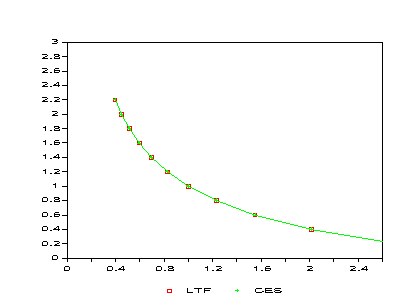
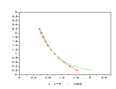
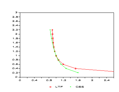
* Evaluate the demand functions:
$LIBINCLUDE qadplot
SET PR Alternative price levels /PR0*PR10/;
PARAMETER
DEMAND(FUNCTION,I,PR) Demand functions
DPLOT(PR,FUNCTION) Plotting output array;
LOOP(II,
LOOP(FUNCTION,
K(N) = YES$SUM(I, SHR(FUNCTION,I,N));
GAMMA = ESUB(FUNCTION,"GAMMA");
SIGMA(K) = ESUB(FUNCTION,K);
S(I,K) = SHR(FUNCTION,I,K);
LOOP(PR,
PRICE(J) = 1;
PRICE(II) = 0.2 * ORD(PR);
$INCLUDE CHKCALIB.GEN
SOLVE CHKCALIB USING MCP;
DEMAND(FUNCTION,II,PR) = D.L(II);
DPLOT(PR,FUNCTION) = D.L(II);
);
);
$LIBINCLUDE qadplot DPLOT PR FUNCTION
);
DISPLAY DEMAND;
A Comparison of Locally-Identical Functions
A Comparison of Locally-Identical Functions
Numerical calibration of NNCES given KLEM elasticities
SET  I  Production input aggregates / K, L, E, M/;  ALIAS (I,J);

* ========================================================================
*       Model-specific data defined here:

PARAMETER
    THETA(I)    Benchmark value shares /K 0.2, L 0.4, E 0.05, M 0.35/

    AUES(I,J)   Benchmark cross-elasticities (off-diagonals) /
                        K.L     1
                        K.E     -0.1
                        K.M     0
                        L.E     0.3
                        L.M     0
                        E.M     0.1 /;
* ========================================================================

SCALAR EPSILON          Minimum value share tolerance /0.001/;

*       Fill in off-diagonals:

AUES(I,J)$AUES(J,I)  =  AUES(J,I);

*       Verify that the cross elasticities are symmetric:

ABORT$SUM((I,J), ABS(AUES(I,J)-AUES(J,I))) " AUES values non-symmetric?";

*       Check that all value shares are positive:

ABORT$(SMIN(I, THETA(I)) LE 0) " Zero value shares are not valid:",THETA;

*       Fill in the elasticity matrices:

AUES(I,I) = 0; AUES(I,I) = -SUM(J, AUES(I,J)*THETA(J))/THETA(I); DISPLAY AUES;

* ========================================================================

*       Define variables and equations for NNCES calibration:

SET     N       Nests within the two-level NNCES function /N1*N4/,
        K(N)    Nests which are in use;

VARIABLES
        S(I,N)        Fraction of good I which enters through nest N,
        SHARE(N)        Value share of nest N,
        SIGMA(N)        Elasticity of substitution within nest N,
        GAMMA           Elasticity of substitution at the top level,
        OBJ             Objective function;

POSITIVE VARIABLES S, SHARE, SIGMA, GAMMA;

EQUATIONS
        SDEF(I)         Nest shares must sum to one,
        TDEF(N)         Nest share in total cost,
        ELAST(I,J)      Consistency with given AUES values,
        OBJDEF          Maximize concentration;

ELAST(I,J)$(ORD(I) GT ORD(J))..

                AUES(I,J) =E=   GAMMA +

                        SUM(K, (SIGMA(K)-GAMMA)*S(I,K)*S(J,K)/SHARE(K));

TDEF(K)..       SHARE(K) =E= SUM(I, THETA(I) * S(I,K));

SDEF(I)..       SUM(N, S(I,N)) =E= 1;

*       Maximize concentration at the same time keeping the elasticities
*       to be reasonable:

OBJDEF..        OBJ =E= SUM((I,K),S(I,K)*S(I,K))

                        - SQR(GAMMA) - SUM(K, SQR(SIGMA(K)));

MODEL   CESCALIB /ELAST, TDEF, SDEF, OBJDEF/;


*       Apply some bounds to avoid divide by zero:

SHARE.LO(N) = EPSILON;

SCALAR  SOLVED  Flag for having solved the calibration problem /0/
        MINSHR  Minimum share in candidate calibration;

SET     TRIES   Counter on the number of attempted calibrations /T1*T10/;

*       We use the random number generator to select starting points,
*       so it is helpful to initialize the seed so that the results
*       will be reproducible:

OPTION SEED=0;

LOOP(TRIES$(NOT SOLVED),

*       Initialize the set of active nests and the bounds:

        K(N) = YES;
        S.LO(I,N) = 0;          S.UP(I,N) = 1;
        SHARE.LO(N) = EPSILON;  SHARE.UP(N) = 1;
        SIGMA.LO(N) = 0;        SIGMA.UP(N) = +INF;

*       Install a starting point:

        SHARE.L(K)  = MAX(UNIFORM(0,1), EPSILON);
        S.L(I,K)    = UNIFORM(0,1);
        GAMMA.L     = UNIFORM(0,1);
        SIGMA.L(K)  = UNIFORM(0,1);

*       Drop any basis information so that we start from scratch:

        SDEF.M(I)     = 0; TDEF.M(K)     = 0; ELAST.M(I,J)  = 0;

        SOLVE CESCALIB USING NLP MAXIMIZING OBJ;

        SOLVED = 1$(CESCALIB.MODELSTAT LE 2);

*       We have a solution -- now see if it is not on a bound:

        IF (SOLVED,

          MINSHR = SMIN(K, SHARE.L(K)) - EPSILON;

          IF (MINSHR EQ 0,

*       Drop nests which have shares equal to EPSILON in the current
*       solution:

            K(N)$(SHARE.L(N) EQ EPSILON) = NO;

            S.FX(I,N)$(NOT K(N)) = 0;
            SHARE.FX(N)$(NOT K(N)) = 0;
            SIGMA.FX(N)$(NOT K(N)) = 0;

            DISPLAY "Recalibrating with the following nests:",K;

            SOLVE CESCALIB USING NLP MAXIMIZING OBJ;

            IF (CESCALIB.MODELSTAT GT 2, SOLVED = 0;);
            MINSHR = SMIN(K, SHARE.L(K)) - EPSILON;
            IF (MINSHR EQ 0, SOLVED = 0;);
          );
        );
);

IF (SOLVED,
        DISPLAY "Function calibrated:",GAMMA.L,SIGMA.L,SHARE.L,S.L;
ELSE
        DISPLAY "Function calibration fails!";
);

$ONTEXT

*==========================================================================

Solution from MINOS obtained on the second try, following an
ITERATION INTERRUPT on the first:

----    151 Function calibrated:


----    151 VARIABLE  GAMMA.L              =        0.300 Elasticity of
                                                          substitution at the
                                                          top level


----    151 VARIABLE  SIGMA.L       Elasticity of substitution within nest N

N3 7.804


----    151 VARIABLE  SHARE.L       Value share of nest N

N1 0.604,    N2 0.266,    N3 0.030,    N4 0.100


----    151 VARIABLE  S.L           Fraction of good I which enters through
                                    nest N

           N1          N2          N3          N4

K                   0.797       0.069       0.133
L       0.960                   0.040
E                                           1.000
M       0.630       0.304                   0.067


*==========================================================================
The following solution is obtained by CONOPT on the second try, following a LOCALLY INFEASIBLE termination on the first problem. Notice that it is identical to the MINOS solution except that the nesting assignments have been permuted:
----    149 Function calibrated:


----    149 VARIABLE  GAMMA.L              =        0.300 Elasticity of
                                                          substitution at the
                                                          top level


----    149 VARIABLE  SIGMA.L       Elasticity of substitution within nest N

N4 7.804


----    149 VARIABLE  SHARE.L       Value share of nest N

N1 0.100,    N2 0.604,    N3 0.266,    N4 0.030


----    149 VARIABLE  S.L           Fraction of good I which enters through
                                    nest N

           N1          N2          N3          N4

K       0.133                   0.797       0.069
L                   0.960                   0.040
E       1.000
M       0.067       0.630       0.304

*==========================================================================

$OFFTEXT
PARAMETER   PRICE(I)    PRICE INDICES USING TO VERIFY CALIBRATION
        AUESCHK(I,J)    CHECK OF BENCHMARK AUES VALUES;

PRICE(I) = 1;

$ontext

$MODEL:CHKCALIB

$SECTORS:
    Y   ! PRODUCTION FUNCTION
    D(I)

$COMMODITIES:
    PY  ! PRODUCTION FUNCTION OUTPUT
    P(I)    ! FACTORS OF PRODUCTION
    PFX ! AGGREGATE PRICE LEVEL

$CONSUMERS:
    RA

$PROD:Y  s:GAMMA.L  K.TL:SIGMA.L(K)
    O:PY        Q:1
    I:P(I)#(K)  Q:(THETA(I)*S.L(I,K))   K.TL:

$PROD:D(I)
    O:P(I)  Q:THETA(I)
    I:PFX   Q:(THETA(I)*PRICE(I))

$DEMAND:RA
    D:PFX
    E:PFX   Q:2
    E:PY    Q:-1
$OFFTEXT
$SYSINCLUDE mpsgeset CHKCALIB

CHKCALIB.ITERLIM = 0;
$INCLUDE CHKCALIB.GEN
SOLVE CHKCALIB USING MCP;
CHKCALIB.ITERLIM = 2000;

SCALAR DELTA /1.E-5/;

ALIAS (I,II);
LOOP(II,

    PRICE(J) = 1;   PRICE(II) = 1 + DELTA;

$INCLUDE CHKCALIB.GEN
    SOLVE CHKCALIB USING MCP;

    AUESCHK(J,II) = (D.L(J)-1) / (DELTA*THETA(II));

);
DISPLAY AUES, AUESCHK;
Calibrating Labor Supply and Savings Demand
This material was published in the MUG newsletter, 8/95.
Following Ballard, Fullerton, Shoven and Whalley (BFSW), we consider a representative agent whose utility is based upon current consumption, future consumption and current leisure. Changes in "future consumption" in this static framework are associated with changes in the level of savings. There are three prices which jointly determine the price index for future consumption. These are:
\(P_I\) the composite price index for investment goods
\(P_K\) the composite rental price for capital services
\(P_C\) the composite price of current consumption.
All of these prices equal unity in the benchmark equilibrium.
Capital income in each future year finances future consumption, which is expected to cost the same as in the current period, PC (static expectations). The consumer demand for savings therefore depends not only on \(P_I\), but also on \(P_K\) and \(P_C\), namely:
\[ P_S=\frac {P_I P_C}{P_K} \]
The price index for savings is unity in the benchmark period. In a counter-factual equilibrium, however, we would expect generally that \(P_S \neq P_I \) . When these price indices are not equal, there is a "virtual tax payment" associated with savings demand.
Following BFSW, we adopt a nested constant-elasticity-of-substitution function to represent preferences. In this function, at the top level demand for savings (future consumption) trades off with a second CES aggregate of leisure and current consumption. These preferences can be summarized with the following expenditure function:
\[ P_U=\big [ \alpha P^{1-\sigma_S}_H + (1-\alpha)P^{1-\sigma_S}_H \big]^{\frac {1} {1-\sigma_S}} \]
Preferences are homothetic, so we have defined \(P_U\) as a linearly homogeneous cost index for a unit of utility. We conveniently scale this price index to equal unity in the benchmark. In this definition, \(\alpha\) is the benchmark value share for current consumption (goods and leisure). \(P_H\) is a compositive price for current consumption defined as:
\[ P_H=\big [ \beta P^{1-\sigma_L}_l + (1-\beta)P^{1-\sigma_L}_C \big]^{\frac {1} {1-\sigma_L}} \]
in which \(\beta\) is the benchmark value share for leisure within current consumption. Demand functions can be written as follows:
\[ \begin{array}{rcll} S=S_0 \bigg ( \frac{P_U}{P_F} \bigg )^{\sigma_S} & \frac{I}{I_0 P_U} , & \end{array} \]
\[ \begin{array}{rcll} C=C_0 \bigg ( \frac{P_H}{P_C} \bigg )^{\sigma_L} & \bigg ( \frac{P_U}{P_H} \bigg )^{\sigma_S} & \frac{I}{I_0 P_U} , & \end{array} \]
and
\[ \begin{array}{rcll} \ell=\ell_0 \bigg ( \frac{P_H}{P_L} \bigg )^{\sigma_L} & \bigg ( \frac{P_U}{P_H} \bigg )^{\sigma_S} & \frac{I}{I_0 P_U} , & \end{array} \]
Demands are written here in terms of their benchmark values ( \(S_0\), \(C_0\) and \(\ell_0\) ) and current and benchmark income ( \(I\) and \(I_0\)).
There are four components in income. The first is the value of labor endowment ( \(E\)), defined inclusive of leisure. The second is the value of capital endowment ( \(K\)). The third is all other income ( \(M\)). The fourth is the value of "virtual tax revenue" associated with differences between the shadow price of savings and the cost of investment.
\[ I=P_L E+P_K K+M+(P_S-P_I) S \]
The following parameter values are specified exogenously:
- \(\zeta =1.75\) is the ratio of labor endowment:
\[ \zeta \equiv E / L_0 \]
where \(L_0\) is the benchmark labor supply. Given \(\zeta\) and L_0 we have:\[ \ell_0 = L_0(\zeta-1) \]
- \(\xi =0.15\) is the uncompensated elasticity of labor supply with respect to the net of tax wage, i.e.
\[ \xi= \frac{\delta L}{\delta P_L}\frac{P_L}{L}= \frac{\delta(E-\ell)}{\delta P_L}\frac{P_L}{L}= -\frac{\delta \ell}{\delta P_L}\frac{P_L}{L} \]
- \(\eta=0.4\) is the elasticity of savings with respect to the return to capital:
\[ \eta \equiv \frac{\delta S}{\delta P_K}\frac{S}{P_K} \]
Shephard's lemma applied at benchmark prices provides the following identities which are helpful in deriving expressions for \(\eta\) and \(\xi\) :\[ \frac{\delta P_U}{\delta P_H}=\alpha , \frac{\delta P_U}{\delta P_S}= 1-\alpha , \frac{\delta P_H}{\delta P_L}=\beta , \frac{\delta P_H}{\delta P_C}=1-\beta , \]
It is then a relatively routine application of the chain rule to show that:\[ \xi = (\zeta-1)\bigg [ \sigma_L +\beta(\sigma_S - \sigma_L)-\alpha \beta (\sigma_S-1)-\frac{E}{I_0} \bigg ] \]
and\[ \eta=\sigma_S \alpha + \frac{K}{I_0} \]
The expression for \(eta\) does not involve \(\sigma_L\) , so we may first solve for \(\sigma_S\) and use this value in determining \(\sigma_L\) :\[ \sigma_S= \frac{\eta-\frac{K}{I_0}}{\alpha} \]
and\[ \alpha_L=\frac{ \frac{\xi}{\xi-1}-\sigma_S\beta(1-\alpha)-\alpha\beta+\frac{E}{I_0}}{1-\beta} \]
A Maquette Illustrating Labor Supply and Savings Demand Calibration
*       Exogenous elasticity:

SCALAR  XI      UNCOMPENSATED ELASTICITY OF LABOR SUPPLY /0.15/,
        ETA     ELASTICITY OF SAVINGS WRT RATE OF RETURN /0.40/,
        ZETA    RATIO OF LABOR ENDOWMENT TO LABOR SUPPLY /1.75/;

*       Benchmark data:

SCALAR  C0      CONSUMPTION /2.998845E+2/,
        S0      SAVINGS /70.02698974/,
        LS0     LABOR SUPPLY / 2.317271E+2/,
        K0      CAPITAL INCOME /93.46960577/,
        PL0     MARGINAL WAGE /0.60000000/;

*       Calibrated parameters:

SCALAR  EL0     LABOR ENDOWMENT
        L0      LEISURE DEMAND
        M0      NON-WAGE INCOME
        I       EXTENDED GROSS INCOME
        ETAMIN  SMALLEST PERMISSIBLE VALUE FOR ETA,
        XIMIN   SMALLEST PERMISSIBLE VALUE FOR XI,
        ALPHA   CURRENT CONSUMPTION VALUE SHARE
        BETA    LEISURE VALUE SHARE IN CURRENT CONSUMPTION
        SIGMA_L ELASTICITY OF SUBSTITUTION WITHIN CURRENT CONSUMPTION
        SIGMA_S ELASTICITY OF SUBSTITUTION - SAVINGS VS CURRENT CONSUMPTION
        TS      SAVINGS PRICE ADJUSTMENT;

*       Convert labor supply into net of tax units:

LS0 = LS0 * PL0;

*       Labor endowment (exogenous):

EL0 = ZETA * LS0;

*       Leisure demand:

L0 = EL0 - LS0;

*       Non-labor, non-capital income:

M0 = C0 + S0 - LS0 - K0;

*       Extended gross income:

I = L0 + C0 + S0;

*       Leisure share of current consumption:

BETA =  L0 / (C0 + L0);

*       Current consumption value share:

ALPHA = (L0 + C0) / I;

*       Calibrated elasticity:

SIGMA_S = (ETA - K0 / I) / ALPHA;
ETAMIN  = K0 / I;
ABORT$(SIGMA_S LT 0) " Error: cannot calibrate SIGMA_S", ETAMIN;

*       Calibrated elasticity of substitution between leisure and consumption:

SIGMA_L = (XI*(LS0/L0)-SIGMA_S*BETA*(1-ALPHA)-ALPHA*BETA+EL0/I)/(1-BETA);
XIMIN = -(L0/LS0) * (- SIGMA_S * BETA * (1-ALPHA) - ALPHA*BETA + EL0/I);
ABORT$(SIGMA_L LT 0) " Error: cannot calibrate SIGMA_L", XIMIN;

DISPLAY "Calibrated elasticities:", SIGMA_S, SIGMA_L;

$ONTEXT

$MODEL:CHKCAL

$COMMODITIES:
        PL
        PK
        PC
        PS

$SECTORS:
        Y
        S

$CONSUMERS:
        RA

$PROD:Y
        O:PC    Q:(K0+LS0-S0)
        I:PL    Q:(LS0-S0)
        I:PK    Q:K0

$PROD:S
        O:PS    A:RA  T:TS
        I:PL

$DEMAND:RA  s:SIGMA_S a:SIGMA_L
        E:PC    Q:M0
        E:PL    Q:EL0
        E:PK    Q:K0
        D:PS    Q:S0
        D:PC    Q:C0  a:
        D:PL    Q:L0  a:
$OFFTEXT
$SYSINCLUDE mpsgeset CHKCAL

S.L = S0;
TS  = 0;

*       VERIFY THE BENCHMARK:

CHKCAL.ITERLIM = 0;
$INCLUDE CHKCAL.GEN
SOLVE CHKCAL USING MCP;

*       CHECK THE LABOR SUPPLY ELASTICITY:

PL.L = 1.001;

CHKCAL.ITERLIM = 0;
$INCLUDE CHKCAL.GEN
SOLVE CHKCAL USING MCP;
*       Compute induced changes in labor supply using the labor market
*       "marginal", PL.M.  This marginal returns the net excess supply of
*       labor at the given prices.  We started from a balanced benchmark,
*       with no change in labor demand (the iteration limit was zero).
*       Hence, PL.M returns the magnitude of the change in labor supply.
*       We multiply by the benchmark wage (1) and divide by the benchmark
*       labor supply (LS0) to produce a finite difference approximation
*       of the elasticity:

DISPLAY "CALIBRATION CHECK -- THE FOLLOWING VALUES SHOULD BE IDENTICAL:", XI;
XI = (PL.M / 0.001) * (1 / LS0);
DISPLAY XI;

PL.L = 1.0;

*       CHECK THE ELASTICITY OF SAVINGS WRT RENTAL RATE OF CAPITAL:

PK.L = 1.001;
PS.L = 1 / 1.001;
TS   = 1 / 1.001 - 1;

CHKCAL.ITERLIM = 0;

*       Compute elasticity of savings with respect to the rental rate of
*       capital.  This requires some recursion in order to account for the
*       effect of changes in savings on effective income.  When PK increases,
*       PS declines -- there is an effective "subsidy" for saving, paid from
*       consumer income.  In order to obtain a difference approximation for
*       the elasticity of savings response, we need to make sure the virtual
*       tax payments are properly handled.  In the MPSGE model, this means
*       that the level value for S must be adjusted so that it exactly equals
*       the savings.  We do this recursively:

SET ITER /IT1*IT5/;


PS.M = 1;
LOOP(ITER$(ABS(PS.M) GT 1.0E-8),

$INCLUDE CHKCAL.GEN
        SOLVE CHKCAL USING MCP;
        S.L = S.L - PS.M;
);

DISPLAY "CALIBRATION CHECK -- THE FOLLOWING VALUES SHOULD BE IDENTICAL:", ETA;
ETA = ((S.L - S0) / 0.001) * (1 / S0);
DISPLAY ETA;