Table of Contents
- Stochastic Programming with Recourse
- Risk Measures with EMP
- Chance Constraints with EMP
Stochastic programs are mathematical programs that involve data that is not known with certainty. Deterministic programs are formulated with fixed parameters, whereas real world problems frequently include some uncertain parameters. Often these uncertain parameters follow a probability distribution that is known or can be estimated. Thus stochastic programs approximate unknown data by probability distributions. The goal is to find some policy that is feasible for all (or almost all) the possible data instances and that maximizes the expectation of some function of the decision variables and the random variables. The EMP framework includes an extension for stochastic programming that allows users to model various stochastic problems as deterministic models, while information about the stochastic structure of the problem, like probability distributions for some data, is specified in the EMP annotations. Thus formulating stochastic programs becomes straightforward.
In the remainder of this chapter we discuss the stochastic programming extension of GAMS EMP. We introduce the basics of stochastic programming with EMP using a two-stage stochastic model and then show how the logic can be extended to multi-stage stochastic problems. In most stochastic problems the expected value of the objective is optimized. The EMP framework facilitates optimizing two additional risk measures: Value at Risk (VaR) and Conditional Value at Risk (CVaR). These alternative risk measures are discussed next. Another type of stochastic programming includes constraints that hold only with certain probabilities. These constrains are called chance constraints (or probabilistic constraints ), they are the topic of the last section on stochastic programming. At the end of each section we give an overview of the EMP annotations that are specific to each topic: stochastic programming with recourse, additional risk measures, and chance constraints. A summary of all EMP keywords for stochastic programming is given in section GAMS EMP Keywords for Stochastic Programming.
Stochastic Programming with Recourse
One way to think about stochastic problems is to require the decision maker to make a decision now and then to minimize the expected costs of the consequences of that decision. This paradigm is called the recourse model. The simplest form of the recourse model has two stages: a decision is made in the first stage, then the realization of the uncertain parameters is revealed at the start of the second stage and recourse actions can be taken given this new information. This simple model can be extended to include more stages. In a multistage problem, a decision is made in the first stage, then some uncertainty is resolved in the second stage and another decision is made based on this new knowledge, then some other uncertainty is resolved and so on. The objective is to minimize the expected costs of the decisions in all stages.
This section is organized as follows. We start with a mathematical formulation of the two-stage stochastic problem with recourse, then show how such problems can be modeled with EMP using a simple example. The uncertain data in this first example follows a discrete distribution, there are just three different scenarios. Continuous distributions are more complex to model. Mostly, they are approximated to discrete distributions by sampling, which is discussed next. The second example illustrates how the modeling approach for a simple two-stage problem can be extended to solve a multi-stage problem. We conclude this section with a description of the EMP annotations for stochastic programs with recourse.
Two-Stage Stochastic Programs: Mathematical Formulation
The simplest form of a stochastic program is the two-stage stochastic linear program with recourse. In mathematical terms it is defined as follows.
Let \(x\in \mathbb{R}^{n}\) and \(y\in \mathbb{R}^{m}\) be two variables and let the set of all realizations of the unknown data be given by \(\Omega\), \(\Omega=\{\omega_1, \dots , \omega_{S} \} \subseteq \mathbb{R}^{r} \), where \(r\) is the number of the random variables representing the uncertain parameters. Then the stochastic program is given by
\begin{equation} \tag {31} \begin{array}{ l l l l l l l l } & \textrm{Min}_{x} & z = & c^{T}x &+& \mathbb{E}[Q(x,\omega)] & &\\ & \textrm{s.t.} & & Ax & & &= & b, \quad \quad \, x \geq 0, \\ \\ \textrm{where} \quad Q(x,\omega) = &\textrm{Min}_{y} & & & & q_{\omega}^T y(\omega) & &\\ & \textrm{s.t.} & & T_{\omega}x &+& W_{\omega} y(\omega) & = & h_{\omega}, \quad \quad y(\omega) \geq 0, \quad \forall \omega \in \Omega. \\ \end{array} \end{equation}
The first two lines define the first-stage problem and the last two lines define the second-stage problem. In the first stage, \(x\) is the decision variable, \(c^T\) represents the cost coefficients of the objective function and \( \mathbb{E}[Q(x,\omega)] \) denotes the expected value of the optimal solution of the second stage problem. In addition, \(A\) denotes the coefficients and \(b\) the right-hand side of the first stage constraints. In the second stage, \(y\) is the decision variable, \(T\) represents the transition matrix, \(W\) the recourse matrix (cost of recourse) and \(h\) the right-hand side of the second stage constraints. Note that all parameters and the decision variable of the second stage are dependent on the specific realization of the stochastic data \(\omega\). The objective variable \(z\) is also a random variable, since it is a function of \( \omega \). As a random variable cannot be optimized, stochastic solvers automatically optimize the expected value of the objective variable \(z\). Note that the EMP framework allows other risk measures to be optimized in addition to the expected value. This is discussed below.
In the first stage, a decision has to be made before the realization of the uncertain data is clear. The optimal solution of the first stage is fixed and only then it will become known which values the uncertain parameters will take. Given the fixed solution of the first stage and the new data, recourse action can be taken in the second stage and the optimal solution determined. Each possible realization of the uncertain data is represented by \(\omega_s \in \Omega\) and is called a scenario. The objective is to find a feasible solution \( x \) that minimizes the total cost, namely the sum of the first-stage costs and the expected second-stage costs.
One of the most common methods to solve a two-stage stochastic LP is to build and solve the deterministic equivalent. Assume that the uncertain parameters follow a (finite) discrete distribution and that each scenario \( \omega_s \) occurs with probability \(P(\omega_s) = p_s\) for all \( s = 1, \dots, S\) and \( \sum_s p_s = 1\). Thus \( \mathbb{E}[Q(x,\omega)] = \sum_s p_s q^{T} y_s \), where \( y_s \) denotes the optimal second-stage decision for the scenario \( \omega_s \). Then the deterministic equivalent can be expressed as follows:
\begin{equation} \tag {32} \begin{array}{ l l l l l l l l l l l } c^T x &+& p_1 q^T y_1 &+& p_2 q^T y_2 &+& \dots &+& p_S q^T y_S & &\\ \textrm{s.t.} & & & & & & & & & & \\ Ax & & & & & & & & &=& b\\ T_1x &+& W_1y_1 & & & & & & &=& h_1 \\ T_2x && & + & W_2y_2 & & & & &=& h_2 \\ \vdots & & & + & & & \ddots & & & & \vdots \\ T_Sx && & & & & & + & W_Sy_S &=& h_S \\ x \in \mathbb{R}^n && y_1 \in \mathbb{R}^m & & y_2 \in \mathbb{R}^m & & & & y_S \in \mathbb{R}^m && \\ \end{array} \end{equation}
Note that for stochastic linear programs the deterministic equivalent is just another (potentially very large) linear program.
A GAMS EMP stochastic model has three parts: the core model, EMP annotations and the dictionary, which contains output-handling information. The core model is a deterministic model, where the uncertain data is given as fixed parameters. Often, the expected value of the probability distribution is chosen.
The annotations contain information about the stochastic features of the model: a specification of the random variables and their distributions, details about the stages and possibly directions concerning sampling.
Given the probability distributions of the random variables, the solvers of stochastic programming models create various scenarios and evaluate them. In the dictionary users specify which results from each scenario are to be stored in standard parameters in order to be accessed later. These three parts of a GAMS EMP stochastic model will become much clearer as they are illustrated in the next subsection.
A Simple Example: The News Vendor Problem
Consider the following simple example adapted from the news vendor model [NBSIMPLE]. A news vendor has to decide early in the morning how many newspapers to buy from a distributor on a particular day in order to sell them to his customers. He knows from experience that the demand will be 45 in 70% of all cases, 40 with a probability of 20% and 50 with a probability of 10%. If the demand is less than the number of newspapers he bought in the morning, the left-over newspapers will be stored in an inventory at a cost per unit. If the demand exceeds his expectations and there are more customers than newspapers, then he will have to pay a penalty. He aims to maximize his profit by selling the newspapers at a higher price than he has bought them. Mathematically, the problem can be expressed as follows:
\begin{equation} \tag{33} \begin{array}{ l l l l l l l l } & \textrm{Max}_{x} & Z(x,D) = - cx + \mathbb{E}[Q(x,D)], & x\geq 0,\\ \\ \textrm{where} \quad Q(x,D) = &\textrm{Max}_{s,i,l} & vs_D - hi_D -pl_D & &\\ & \textrm{s.t.} & x - s_D - i_D = 0 \\ & & s_D + l_D = D, & s_D, i_D, l_D\geq 0\\ \end{array} \end{equation}
where
- the variable \(x\) denotes the number of newspaper bought in the morning,
- \(c\) is the cost per newspaper,
- \(D\) is a random variable that denotes the uncertain demand; the set of all realizations of \(D\) is given by \(\Omega = \{d_1, d_2, d_3\}\), with \(d_1=45\), \(d_2=40\) and \(d_3=50\), and the respective probabilities \(p_1=0.7\), \(p_2=0.2\) and \(p_3=0.1\),
- the variable \(s\) denotes the number of newspapers that are sold,
- \(v\) is the selling price,
- the variable \(i\) denotes the number of newspapers that could not be sold, in case the demand turned out to be less than expected,
- \(h\) is the holding cost in the inventory per unit,
- the variable \(l\) denotes the unsatisfied demand, in case the demand turned out to be higher than expected,
- \(p\) is the penalty per unit of unsatisfied demand.
Note that \(x\) is the first-stage decision variable and the variables \(s\), \(i\) and \(l\) are the second-stage decision variables. The second-stage decision variables are dependent on \(D\). An overview of the stages in this problem is given in the following table:
| 1st Stage Decision Variable | 2nd Stage Decision Variable; \(\Omega = \{d_1, d_2, d_3\}\) | Probabilities |
|---|---|---|
| \(x\) | \(y_{d_1} = (s_{d_1}, l_{d_1}, i_{d_1})\) | Scenario 1: \(p_1 = 0.7\) |
| \(x\) | \(y_{d_2} = (s_{d_2}, l_{d_2}, i_{d_2})\) | Scenario 2: \(p_2 = 0.2\) |
| \(x\) | \(y_{d_3} = (s_{d_3}, l_{d_3}, i_{d_3})\) | Scenario 3: \(p_3 = 0.1\) |
Table 3: Two stages in the News Vendor Problem
Observe that the decision \(x\) has to be made before the realization of the demand \(D\) is known. Given the uncertainty of the demand, we aim to maximize the expected value of the profit, denoted by \(\mathbb{E}[Z(x,D)]\). The expected value of the profit is the profit on average. Note that as we have a finite number of scenarios and their probabilities are known, the expected value of the profit \(\mathbb{E}[Z(x,D)]\) can be expressed as a weighted sum:
\begin{equation} \tag{34} \begin{array}{l l} \mathbb{E}[Z(x,D)] = & -cx + \mathbb{E}[Q(x,D)] \\ & -cx + \sum_{k=1}^3 p_kQ(x,d_k). \end{array} \end{equation}
Note that in this example there are no first stage equations \(Ax=b\).
The core model is the first part of the respective GAMS EMP model:
Variable  z      "profit";
Positive Variables
          x      "units bought"
          i      "inventory"
          l      "lost sales"
          s      "units sold";

Scalars   c      "purchase costs per unit"         / 30 /
          p      "penalty shortage cost per unit"  /  5 /
          h      "holding cost per leftover unit"  / 10 /
          v      "revenue per unit sold"           / 60 /
          d      "demand, random parameter"        / 45 /;

Equations profit "profit to be maximized"
          row1   "demand = UnitsSold + LostSales"
          row2   "inventory = UnitsBought - UnitsSold";

profit..  z =e= v*s - c*x - h*i - p*l;
row1..    d =e= s + l;
row2..    i =e= x - s;

Model nv / all /;
Observe that the model is defined in the usual way. In particular, the demand d is modeled as a fixed parameter.
The EMP annotations are the second part. Here we specify the stochastic structure:
File emp / '%emp.info%' /;
put emp '* problem %gams.i%'/;
$onput
randvar d discrete 0.7 45 0.2 40 0.1 50
stage 2 i l s d
stage 2 Row1 Row2
$offput
putclose emp;
First, we define the parameter d to be a random variable using the EMP keyword randvar and we specify the probability distribution. The EMP keyword discrete indicates that d follows a discrete distribution: with probability 0.7 it takes a value of 45, with probability 0.2 it takes a value of 40, and with probability 0.1 it takes a value of 50.
- Note
- If the sum of the probabilities of a discrete distribution is smaller or larger than 1, the EMP framework will automatically normalize the probabilities so that the sum equals 1 and a corresponding remark will appear in the log and listing file.
Observe that continuous distributions are also possible, see section Random Variables with Continuous Distributions below for details.
Secondly, we specify which variables and equations belong to stage 2 using the EMP keyword stage. Note that the variables and equations that are not listed in the annotations are automatically assigned to a stage, by default stage 1 (this could be changed using the EMP keyword stageDefault). Only the objective variable (in this case Z) and the objective equation (profit) are assigned to the highest stage specified instead (stage 2 in this example). Observe that \(Z\) is in fact a random variable since it is a function of the random variable \(D\). As such it cannot be optimized directly, EMP implicitly maximizes the expected value of \(Z\). This might lead to some confusion since the expected value of \(Z\) belongs to stage 1. We show in section Expected Value Revisited how to specify more clearly the fact that we are maximizing \(\mathbb{E}(Z)\).
All keywords that can be used in EMP annotations in the context of stochastic programming are introduced in subsequent examples and they are summarized in section GAMS EMP Keywords for Stochastic Programming.
The dictionary with output-handling information and the solve statement are the third part of the model. After solving a stochastic programming model, only the solution of the expected value problem may be accessed via the regular .l and .m fields. The results of the scenarios that were created and evaluated by the stochastic solvers may be stored in standard parameters in the following way:
Set scen           "scenarios" / s1*s3 /;
Parameter
     s_d(scen)     "demand realization by scenario"
     s_x(scen)     "units bought by scenario"
     s_s(scen)     "units sold by scenario"
     s_rep(scen,*) "scenario probability"   / #scen.prob 0/;

Set dict / scen .scenario.''
           d    .randvar .s_d
           s    .level   .s_s
           x    .level   .s_x
           ''   .opt     .s_rep /;

solve nv max z use EMP scenario dict;
display s_d, s_x, s_s, s_rep;
The size of the set scen defines the maximal number of scenarios we are willing to store results for. It does not have to match the number of scenarios that are actually generated in the solution process. Assume that the size of the set scen is \(n\) and \(n\) is smaller than the number of generated scenarios. In this case only the results for the first \(n\) scenarios will be stored. On the other hand, if the size of scen is larger than the number of generated scenarios, then the positions of the surplus elements of scen will be empty in the parameters (e.g. s_d).
The elements of the three-dimensional set dict determine which scenario-dependent values will be stored. The set contains mapping information between the symbols in the model in the first position and the symbols in which scenario solution information is stored in the third position. The type of storing is specified in the second position. The following entries are allowed:
| Label | Description |
|---|---|
level | Stores the level values of a scenario solution of a variable or equation. |
marginal | Stores the marginal values of a scenario solution of a variable or equation. |
randvar | Stores the realization of a random variable. |
opt | Stores the probability of each scenario. |
scenario | The symbol in the first position of the tuple is used as the scenario index. |
Table 4 Entries in the second position of the tuples in the scenario dictionary
- Attention
- The first two tuples in the set
dictare mandatory, all other elements of the set are optional. If one of the first two tuples is missing, the stochastic model cannot be solved and an error will be generated.
In the example above, we store the realization for each scenario of the random variable d in the parameter s_d, the level values of the variables s and x in the parameters s_s and s_x respectively and the actual probability of each scenario in the parameter s_rep.
- Note
- Storing and retrieving the actual probabilities of the scenarios may be particularly relevant if the probabilities have been normalized such that their sum equals 1.
Finally, the solve statement needs to be adjusted: we use the model type EMP and add scenario dict to indicate that a stochastic problem is to be solved.
Random Variables with Continuous Distributions
Now we assume that the random variable \(D\) in the example above has a continuous distribution, say a Normal distribution with mean 45 and standard deviation 10. The structure of the problem remains unchanged, the only difference is that the set \(\Omega\), that is the set of all realizations of \(D\), contains an infinite number of scenarios. There are various ways of modeling this. For example, a sampling procedure implemented in the solver can be used: a finite number of scenarios is generated to approximate \(\Omega\) and thus the problem is converted to a problem with a finite discrete distribution.
We can model a continuous distribution of the random variable in GAMS EMP by changing the annotations in the following way:
randvar d normal 45 10
Note that currently only the solver LINDO has implemented a sampling procedure for parametric distributions so that it can solve such a problem directly. If the solver DE is used, the sampling can be performed by the LINDO system behind the scenes. More details about sampling are given in the next section. All parametric distributions that can be modeled are listed in Table 5 .
| Distribution | Parameter 1 | Parameter 2 | Parameter 3 |
|---|---|---|---|
| Beta | shape 1 | shape 2 | |
| Cauchy | location | scale | |
| Chi_Square | deg. of freedom | ||
| Exponential | lambda | ||
| F | deg. of freedom 1 | deg. of freedom 2 | |
| Gamma | shape | scale | |
| Gumbel | location | scale | |
| Laplace | mean | scale | |
| Logistic | location | scale | |
| LogNormal | mean | std dev | |
| Normal | mean | std dev | |
| Pareto | scale | shape | |
| StudentT | deg. of freedom | ||
| Triangular | low | mid | high |
| Uniform | low | high | |
| Weibull | shape | scale | |
| Binomial | n | p | |
| Geometric | p | ||
| Hyper_Geometric | total | good | trials |
| Logarithmic | p-factor | ||
| Negative_Binomial | failures | p | |
| Poisson | lambda |
Table 5: Parametric distributions supported by LINDO
Recall that there are two ways to specify that a specific solver should be used (that is not the default solver for the problem type): with a command line parameter (e.g. emp=lindo) and with an option statement (e.g. option emp = lindo;).
Examples with random variables that follow parametric distributions include the multistage example below (three random variables with Gamma distributions) and the production model [PRODSP3] in the GAMS EMP Model Library (one random variable that follows a Normal distribution and one random variable that is uniformly distributed).
Sampling
Currently, only the solver LINDO has the ability to perform sampling for parametric distributions directly. Note that LINDO generates 6 samples by default and users need a LINDO license for sample sizes larger than 10 (smaller sample sizes are included in the demo version, but just for certain distributions). Also, changing the default variance reduction method requires a valid LINDO license. There are three ways to customize sampling: including additional information in the EMP annotations, generating a sample with the LINDO library lsadclib (these two options allow to pass on the samples to other solvers with EMP SP capabilities) and setting various options in the solver LINDO. We discuss each method in more detail in the next three subsections.
Customizing Sampling in the EMP Annotations
The EMP framework provides two keywords to facilitate sampling: sample and setSeed. The keyword sample allows users to specify the size of the sample in the EMP annotations. Consider the following example:
randvar d normal 45 10
sample d 9
The second line specifies that the size of the sample of the distribution of the random variable \(D\) is 9. Note that currently the LINDO Sampling Library is used for this sampling. If the solver DE is used and a parametric distribution for the random variable is specified, the second line with the keyword sample is mandatory. Otherwise the following error message will appear:
*** Only random variables with sampled continuous distributions supported.
In addition to specifying the size of the sample, information about a mathematical variance reduction method may be added in the line that starts with the keyword sample. Variance reduction is a procedure used to increase the precision of the estimated values from the distribution. LINDO provides three methods for reducing the variance: Monte Carlo sampling, Latin Square sampling and Antithetic sampling. We illustrate with an example.
Consider a stochastic model with four random variables: \(E\), \(F\), \(G\) and \(H\). Assume that \(E\) follows a Normal distribution with mean 23 and standard deviation 5, \(F\) follows a Normal distribution with mean 37 and standard deviation 8, \(G\) is uniformly distributed on the interval \([0,1]\) and \(H\) is binomially distributed with \(n=100\) and \(p=0.55\). We wish that three variance reduction methods are applied: Antithetic sampling is to be used for \(E\) and \(F\), Monte Carlo sampling for \(G\) and Latin Square sampling for \(H\). We insert the following lines in the EMP annotations:
randvar e normal 23 5
randvar f normal 37 8
randvar g uniform 0 1
randvar h binomial 100 0.55
sample e f 10 method1
sample g 12 method2
sample h 8 method3
First, the random variables and their distributions are defined. Next, details about the sampling procedures are given. Note that the keyword sample can take more than one random variable if the sample size and the variance reduction method for these random variables are identical. We need to add the following lines before the solve statement to specify the content of method1, method2 and method3 (we assume that the name of the model is nv):
$onecho > lindo.opt
SVR_LS_ANTITHETIC=method1
SVR_LS_MONTECARLO=method2
SVR_LS_LATINSQUARE=method3
$offecho
nv.optfile=1;
If Latin Square sampling should also be used for \(E\) and \(F\), we would simply change the EMP annotations to replace the label method1 with the label method3. For more details on variance reduction methods, please consult the LINDO manual.
In addition, the EMP keyword setSeed may be used to further customize the sampling procedure:
setSeed <seed>
This line sets the seed (an integer number) for the random number generator of the sampling routines. If setSeed is used in the EMP annotations, the seed will be set once before all samples are generated. Please note that setSeed only works with a valid LINDO license.
Separating Sampling and Solving
Users may want to sample from a distribution with the LINDO system and solve the model with another solver, say DE. This is possible with the sampling routines from the LINDO Sampling Library lsadclib. We could solve the news vendor model by first drawing a sample from a Normal distribution with mean 45 and standard deviation 10 and then using the sample in the EMP annotations. The GAMS code for sampling from a Normal distribution where the sample size is 9 follows:
$funclibin msllib lsadclib

Function setSeed         / msllib.setSeed /
         sampleNormal    / msllib.sampleLSNormal /
         getSampleValues / msllib.getSampleValues /;

Scalar k;
k = sampleNormal(45,10,9);

Set g /1*9/; parameter sv1(g);
loop(g,
   sv1(g) = getSampleValues(k);
);
display sv1;
The directive in the first line makes the LINDO sampling library available, msllib is the internal library name (see also $funcLibIn for more information). For further details and a list of the available probability distributions, see section The LINDO Sampling Library.
In the following lines we demonstrate how the sample is used in the EMP annotations:
File emp / '%emp.info%' /;
put emp;
put 'randvar d discrete '; loop(g, put (1/card(g)) ' ' sv1(g) ' ');
$onput
stage 2 I L S d
stage 2 Row1 Row2
$offput
putclose emp;
Note that the third line states that the random variable \(D\) follows a discrete distribution and the probabilities and values are taken from the previously generated sample. The other lines of the annotations remain unchanged.
Sampling Options for the Solver LINDO
There are some customizable sampling options in LINDO. Users could control the number of sampled scenarios by setting any of the following LINDO/SP options in the file LINDO options file lindo.opt:
STOC_NSAMPLE_PER_STAGE      - list of sample sizes per stage (starting at stage 2)
STOC_NSAMPLE_SPAR           - common sample size per stochastic parameter
STOC_NSAMPLE_STAGE          - common sample size per stage
For example, we could insert the following three lines before the solve statement:
option emp = lindo;
$echo STOC_NSAMPLE_STAGE = 100 > lindo.opt
nv.optfile = 1;
The first line directs GAMS to solve models of the type emp with the LINDO solver. The second line writes STOC_NSAMPLE_STAGE = 100 to the file lindo.opt, it communicates to the solver to generate 100 samples per stage. The third line informs GAMS to use the solver option file (i.e. lindo.opt).
The following example shows how to use large samples and instruct LINDO to use a Benders decomposition algorithm to tackle the problem:
$onecho > lindo.opt
STOC_MAX_NUMSCENS = 1000000
STOC_NSAMPLE_STAGE = 40
STOC_METHOD = 1
$offecho
In the second line we ensure that the maximum number of scenarios is large enough. The options in the following lines state the sample size and determine the stochastic method to be used (1 means Nested Benders Decomposition). For further details on LINDO options, please consult the LINDO user manual.
Multistage Stochastic Programming Example
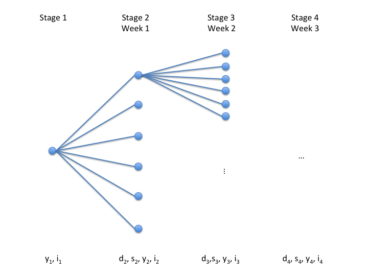
The modeling principles for two-stage stochastic models can be easily extended to multistage stochastic models. At the beginning of each stage some uncertainty is resolved and recourse decisions or adjustments are made after this information has become available. At the point where decisions are made only outcomes of the current stage and previous stages are available. This logic can be pictured schematically as follows:
\begin{equation} \begin{split} \underbrace{\text{Make decision}}_{\text{Stage 1}} \rightarrow \underbrace{\text{Random Variable is realized} \rightarrow \text{Make decision}}_{\text{Stage 2}} \\ \rightarrow \dots \rightarrow \underbrace{\text{Random Variable is realized} \rightarrow \text{Make decision}}_{\text{Stage n}} \end{split} \end{equation}
Observe that random variables which are realized in stage \(k\) are fixed parameters in stage \(k+1\) and following; stage 1 random variables are in fact simply given deterministic values and will create a warning or an error dependent on the solver selected.
Consider an inventory problem. At the end of each week the decision how many hats should be bought in order to satisfy the stochastic demand in the following week must be made. The aim is to maximize the profit. We assume that the stochastic demand can be modeled using a Gamma distribution. The planning horizon is 3 weeks. Before the first week starts an initial purchase decision has to be made and the goods are stored in the inventory for use in week 1. At this point only the distribution of the demand of the first week is known. During the first week the actual demand is revealed and some items that were stored in the inventory are sold. Some items may be left over; they are stored as the inventory for the second week. In addition, a purchase decision for the second week has to be made given the size of the inventory and the distribution of the demand in the second week. Again, the actual demand is revealed in the course of the second week. The same holds for the third week.
We will model the problem with 4 stages, where the first stage corresponds to the preparation time before the first week, the second stage corresponds to decisions made in the first week, the third stage corresponds to decisions made in the second week and the fourth stage corresponds to decisions made in the third week. Let \(t\) denote the stages. Note that while the stages range from \(t=1\) to \(t=4\), demand variables are realized only at \(t=2\) to \(t=4\). Let \(y_t\) be the amount bought and \(i_t\) the amount stored at the end of each stage and let \(D_t\) denote the demand in each week and \(s_t\) the amount sold each week. Note that we denote the demand with a capital \(D\) since it is a random variable. Let \(\alpha=10\) be the cost per hat bought, \(\beta=20\) the revenue per hat sold and \(\delta=4\) the storage cost per unit. Further, in the storage facility a maximum of \(\kappa=5000\) hats can be stored.
Mathematically, this problem can be expressed as follows:
\begin{equation}\tag{35} \begin{array}{lll} \textrm{Max}_{s_t, y_t, i_t} & z = - \alpha y_1 -\gamma i_1 + \mathbb{E}[ \textrm{Max} \quad \beta s_2(D_2) - \alpha y_2(D_2) - \delta i_2(D_2) + \dots + \\ & \mathbb{E} [\textrm{Max} \quad \beta s_4(D_4) + - \alpha y_4(D_4) - \delta i_4(D_4) ] \dots ] \\ \textrm{s.t.} & i_1 = y_1 \\ & i_{t-1} + y_t = s_t + i_t \\ & s_t \leq i_{t-1} \\ & s_t \leq D_t \\ & i_t \leq \kappa\\ & y_1, i_1, s_t, y_t, i_t \geq 0,\\ \end{array} \end{equation}
where \(t = 2, \dots, 4\) and \(D_t\) follows a Gamma distribution. Note that \(s_t\), \(y_t\) and \(i_t\) depend on the realization of \(D_t\).
As discussed above, the solvers use a sampling procedure to approximate a problem with a continuous random variable by a problem with a discrete distribution. Figure 1 illustrates the stages assuming a sample size of 6 (per stage). Note that this results in a total of \(6^3 = 216\) scenarios.
The problem can be modeled with GAMS EMP as follows:
* Core Model
Set t            "stages" / 1*4 /;
Set st(t)        "stages where sales occur" / 2*4 / ;

Positive Variables
     y(t)        "units to be bought in time period t"
     i(t)        "ending inventory in period t"
     s(t)        "units sold in time period t" ;
Free Variable
     profit ;

Scalars
    kappa        "capacity of storage building"                   / 5000 /
    alpha        "cost per unit bought"                           /   10 /
    beta         "revenue per unit sold"                          /   20 /
    delta        "cost per unit stored at the end of time period" /    4 / ;

Parameters
     k           "shape of demand (1st parameter of gamma distribution)" / 16         /
     d_theta(st) "scale of demand (2nd parameter of gamma distribution)" / 2 208.3125
                                                                           3 312.5
                                                                           4 125      /
     d(st)       "demand" ;

d(st) = k * d_theta(st);

Equations
     defprofit   "definition of profit"
     balance(t)  "balance equation"
     sales1(st)  "sales cannot exceed demand"
     sales2(t)   "sales cannot exceed inventory of previous time period" ;

defprofit..        profit =e= sum(t, beta * s(t)$st(t) - alpha * y(t) - delta * i(t));
balance(t)..       i(t-1) + y(t) =e= s(t)$st(t) + i(t) ;
sales1(st)..       s(st) =l= d(st);
sales2(t)$st(t)..  s(t) =l= i(t-1);

i.up(t) = kappa;
Model inventory /all/;

* EMP Annotations
File emp / '%emp.info%' /;
put emp; emp.nd=6;
put "randvar d('2') gamma ", k d_theta('2') /;
put "randvar d('3') gamma ", k d_theta('3') /;
put "randvar d('4') gamma ", k d_theta('4') /;
$onput
stage 1 y('1') i('1') balance('1')
stage 2 y('2') d('2') s('2') i('2') balance('2') sales1('2') sales2('2')
stage 3 y('3') d('3') s('3') i('3') balance('3') sales1('3') sales2('3')
stage 4 y('4') d('4') s('4') i('4') balance('4') sales1('4') sales2('4')
$offput
putclose emp;

* Dictionary
Set scen          "scenarios" / s1*s216 /;
Parameters
     s_d(scen,st) "demand realization by scenario"
     s_y(scen,t)  "units bought by scenario"
     s_s(scen,t)  "units sold by scenario"
     s_i(scen,t)  "units stored by scenario" ;

Set dict /
   scen .scenario.''
   d    .randvar .s_d
   s    .level   .s_s
   y    .level   .s_y
   i    .level   .s_i  /;

option emp=lindo;
solve inventory max profit using emp scenario dict;
display s_d, s_s, s_y, s_i;
Observe that in the core problem the values of the demand d(t) are replaced by the expected values of the random variable \(D_t\) which follows a Gamma distribution. Note that as expected, in stage 1 we have only the variables y and i, but no variables s and d. Recall that currently only the solver LINDO can solve models with parametric distributions, see sections Random Variables with Continuous Distributions and Sampling for more information.
EMP Syntax for Stochastic Programs with Recourse
The general syntax of the EMP annotations used to specify stochastic problems with recourse is as follows:
[randvar rv discrete prob val {prob val}]
[randvar rv distr par {par}]
[jrandvar rv rv {rv} prob val val {val} {prob val val {val}}]
[setSeed number]
[sample  rv1 [rv2 ... rvn] sampleSize [varRedMethod]]
stage stageNo rv | equ | var {rv | equ | var}
{stage stageNo rv | equ | var {rv | equ | var}}
[stageDefault stageNo]
The first three lines present three ways to specify random variables: a single random variable with a discrete distribution, a single random variable with a parametric distribution and joint random variables with discrete distributions. Note that randvar, jrandvar and discrete are EMP keywords. The distribution of single discrete random variables is defined by pairs of the probability prob of an outcome and the corresponding realization val, see example above. The distribution of parametric random variables is defined by the name of the distribution dist and the respective parameter(s) par. An overview of all supported parametric distributions can be found in Table 5. All possible values for distr and the related parameters par are listed there. The keyword jrandvar is used to define discrete random variables that are jointly distributed. At least two random variables must be named. For an example, see the news vendor model [NBDISCJOINT].
- Note
- At least one random variable must be defined and all three ways to define random variables may appear in the EMP annotations. See the scheduling model [AIRLIFT] for an example with both, a discrete random variable and a continuous random variable.
The keywords setSeed and sample are optional. The seed for the random number generator may be set with setSeed. The random number generator is used for the sampling routines that are called with the keyword sample. If setSeed is used, the seed will be set once before all samples will be generated. The keyword sample is followed by the name of the respective random variable, the sample size (a number) and - optionally - a variance reduction method. Note that the random variable must have been previously declared to follow a parametric distribution. Note further, that the sample size of more than one random variable may be customized simultaneously. Observe that the default sample size is 6. For details on available variance reduction methods, see section Customizing Sampling in the EMP Annotations.
- Note
- A valid LINDO license is required to use the keywords
setSeedandsample. The keywordsamplemay be used with a demo or community version of the LINDO license, but it is limited to the Normal and Binomial distributions with a maximum sample size of 10 and the variance reduction method cannot be changed. - If a parametric distribution is used with any solver but LINDO, the keyword
sampleis mandatory, see above for details.
- A valid LINDO license is required to use the keywords
With the keyword stage random variables, variables and equations are assigned to their respective stages, where StageNo defines the stage number. Note that the default stage for all random variables, equations and variables is 1, except for the objective equation and variable. The default for those is the highest stage in the problem.
With the keyword stageDefault one can change the default stage to which symbols get assigned if they are not listed with a stage keyword explicitly.
Risk Measures with EMP
The literature on stochastic programming usually assumes that the expected value of the objective is optimized. The EMP tool follows this trend and implicitly optimizes the expected value. However, there are other risk measures that could be taken into consideration and that are frequently used in practice, particularly in finance. For example, a fund manager might be more interested in the expected value of the 10% worst cases of the projected wins than in the expected value of the overall distribution. The expected value of a partition of the distribution at one tail is called Conditional Value at Risk. The EMP framework provides special keywords to facilitate optimizing this risk measure. On a more abstract level, risk measures can be understood as mechanisms to evaluate the effects of uncertainty in the underlying system on the outcomes of interest. They can be used to modify the distribution of outcomes.
Using the example of an investor who wishes to balance expected rewards and the risk of loss when she decides how to allocate assets in a portfolio, we explore how stochastic optimization problems involving risk measures can be modeled with EMP. Note that this example is adapted from the stochastic portfolio model [PORTFOLIO]. For simplicity of exposition, we only describe two-stage models here. In the examples that follow, the period \((0,T)\) is the period between investing in a portfolio of assets and return from this portfolio.
We first present the example problem and introduce a new EMP keyword to model the expected value explicitly. Then we introduce and discuss Value at Risk (VaR) and Conditional Value at Risk (CVaR). At the end of this section, we give a summary of the EMP annotations that are specific to risk measures.
- Note
- The stochastic extension of EMP facilitates the optimization of a single risk measure or a combination of risk measures (for example, the weighted sum of Expected Value and CVaR). In addition, the modeler can choose to trade off risk measures.
Expected Value Revisited
Suppose an investor has the opportunity to invest a certain amount in three assets. She is given the probability distribution in Table 6 that links each asset with a possible return at time \(T\). The question arises how she should allocate her funds between the three assets at time 0 in order to maximize her expected return at time \(T\).
| Scenario | Probability | ATT | GMC | USX |
|---|---|---|---|---|
| s1 | 1/12 | 1.300 | 1.225 | 1.149 |
| s2 | 1/12 | 1.103 | 1.290 | 1.260 |
| s3 | 1/12 | 1.216 | 1.216 | 1.419 |
| s4 | 1/12 | 0.954 | 0.728 | 0.922 |
| s5 | 1/12 | 0.929 | 1.144 | 1.169 |
| s6 | 1/12 | 1.056 | 1.107 | 0.965 |
| s7 | 1/12 | 1.038 | 1.321 | 1.133 |
| s8 | 1/12 | 1.089 | 1.305 | 1.732 |
| s9 | 1/12 | 1.090 | 1.195 | 1.021 |
| s10 | 1/12 | 1.083 | 1.390 | 1.131 |
| s11 | 1/12 | 1.035 | 0.928 | 1.006 |
| s12 | 1/12 | 1.176 | 1.715 | 1.908 |
Table 6: Return by scenario
Mathematically, the problem can be expressed as follows:
\begin{equation}\tag{36} \begin{array}{ll} \textrm{Max} & \mathbb{E}[R] \\ \textrm{s.t} & R = \sum_j w_j v_j\\ & \sum_j w_j = 1 \\ & w_j \geq 0,\\ \end{array} \end{equation}
where the variable \(R\) denotes the return and is a function of the random variable \(v\), \(\mathbb{E}[R]\) is the expected return, \(w_j\) is the weight associated with each asset \(j\), and \(v_j\) is the return of each asset \(j\). The weights can also be interpreted as proportions of the amount to be invested, their sum must equal 1. Note that \(w_j\) is the decision variable in this problem. Note further, that \(v_j\) is a random variable that depends on which scenario is realized.
We present two different ways to model this problem in GAMS EMP: in the first version the expected value of the return is modeled implicitly and in the second version it is modeled explicitly. Both models have two stages, in the first stage the weights are chosen without knowing which scenario will be realized, in the second stage the 12 scenarios are taken into account. We start with the part of the code where the data is given. It is named data.gms and it will be included in all models in this section.
Sets   j       "assets"     / att, gmc, usx /
       s       "scenarios"  / s1*s12 / ;

Table vs(s,j) "scenario returns from assets"
     att     gmc     usx
 s1  1.300   1.225   1.149
 s2  1.103   1.290   1.260
 s3  1.216   1.216   1.419
 s4  0.954   0.728   0.922
 s5  0.929   1.144   1.169
 s6  1.056   1.107   0.965
 s7  1.038   1.321   1.133
 s8  1.089   1.305   1.732
 s9  1.090   1.195   1.021
s10  1.083   1.390   1.131
s11  1.035   0.928   1.006
s12  1.176   1.715   1.908 ;

Parameters
      v(j)    "return from assets "
      p(s)    "probability" / #s [1/card(s)] / ;

v(j) =  sum(s, vs(s,j))/card(s);
The first model is similar to the two-stage example model above, the fact that the expected return is being maximized is not stated explicitly but is only implied:
* Core Model
$include data.gms
Variables
      r       "value of portfolio under each scenario"
      w(j)    "portfolio selection" ;
Positive Variables
      w ;

Equations
      defr    "return of portfolio"
      budget  "budget constraint" ;

defr..     r =e= sum(j, v(j)*w(j));
budget..   sum(j, w(j)) =e= 1;

Model portfolio / all /;

* EMP Annotations
File emp / '%emp.info%' /;
emp.nd=4;
put emp '* problem %gams.i%'
    / 'stage 2 v r defr'
    / "jrandvar v('att') v('gmc') v('usx')"
loop(s,
  put / p(s) vs(s,"att") vs(s,"gmc") vs(s,"usx"));
putclose emp;

* Dictionary
Parameters
      s_v(s,j) "return from assets by scenario"
      s_r(s)   "return from portfolio by scenario" ;

Set   dict / s  .scenario.''
             v  .randvar .s_v
             r  .level   .s_r /;

solve portfolio using emp max r scenario dict;
display s_v, s_r;
As usual, the core model is defined first and the specifications relating to the stochastic structure of the model are written to the file emp.info. Note that the statement emp.nd=4 ensures that 4 decimal places are used for the values of the parameter vs. In the first line of the EMP annotations, the variables v and r and the equation defr are assigned to the second stage. Note that the other variables and equations (in this case, the variable w and the equation budget) are automatically assigned to the first stage. In the second line of the annotations, the EMP keyword jrandvar is used to declare that v('att'), v('gmc') and v('usx') are joint random variables, i.e. they are jointly distributed (thus we have 12 scenarios and not 12*12*12=1728 scenarios). The respective probabilities and values are specified with a loop statement. Observe that the syntax of the solve statement suggests that the return r is maximized. However, r is in fact a random variable, since it is a function of random variables, so actually the expected return is maximized.
In the second model we introduce a new variable for the expected return, evr. This new variable is linked to the EMP keyword ExpectedValue in the annotations, thus it is made explicit that the expected value of the return is optimized.
* Core Model
$include data.gms
Variables
      r       "value of portfolio under each scenario"
      w(j)    "portfolio selection"
      evr     "expected value of r"
      obj     "objective variable" ;
Positive Variables
      w ;

Equations
      defr    "return of portfolio"
      budget  "budget constraint"
      defobj  "objective equation" ;

defr..     r =e= sum(j, v(j)*w(j));
budget..   sum(j, w(j)) =e= 1;
defobj..   obj =e= evr;

Model portfolio / all /;

* EMP Annotations
File emp / '%emp.info%' /;
emp.nd=4;
put emp '* problem %gams.i%'
    / 'ExpectedValue r evr'
    / 'stage 1 obj defobj evr'
    / 'stage 2 v defr r'
    / "jrandvar v('att') v('gmc') v('usx')"
loop(s,
  put / p(s) vs(s,"att") vs(s,"gmc") vs(s,"usx"));
putclose emp;

* Dictionary
Parameters
      s_v(s,j) "return from assets by scenario"
      s_r(s)   "return from portfolio by scenario" ;

Set   dict / s  .scenario.''
             v  .randvar .s_v
             r  .level   .s_r /;

solve portfolio using emp max obj scenario dict;
In the EMP annotations, the EMP keyword ExpectedValue is followed by the variable r and the variable evr. In this way the variable evr is declared to be the expected value of the (random) variable r. Note that the new variables evr and obj belong to stage 1 and the variable evr is maximized (via obj). The remainder of the annotations and the code referring to the output-handling information in the dictionary are the same like in the first model. Both models have the same solution. We prefer the second model since the syntax is more explicit and clearer.
Observe that the keyword ExpectedValue is particularly useful if users wish to model an objective that is the weighted sum of several risk measures, thus trading-off different risk measures. An example with the weighted sum of the expected value and Value at Risk as objective and an example with the weighted sum of the expected value and Conditional Value at Risk as objective are given below.
Value at Risk (VaR)
The Value at Risk (VaR) is the value of the distribution at a given cut-off point; for example, the value of the standard Normal distribution at the point \(x\) such that 95% of the distribution is to the left. In this subsection we introduce the notion of VaR in more detail by developing a mathematical formulation, demonstrating how VaR can be modeled with GAMS EMP using a simple example and showing how to optimize the weighted sum of the expected value and VaR.
VaR: Mathematical Formulation
Suppose \(G(x, \xi)\) is a real valued function of the decision vector \(x\) and a random data vector \(\xi\) and that it denotes the loss function of a portfolio of assets. We aim to restrict potential losses and so we choose a portfolio composition such that the loss only exceeds a certain threshold \(\gamma\) ( \(\gamma \in \mathbb{R}\)) with a probability smaller or equal to \(\alpha\), \(\alpha \in (0,1)\), where \(\alpha\) is small. This condition can be modeled as a chance constraint and has the following form:
\begin{equation} \tag{37} P(G(x, \xi) > \gamma) \leq \alpha \end{equation}
It is easy to see that this can be written in the following way:
\begin{equation} \tag{38} \label{eq_G_minus_gamma} P(G(x, \xi) - \gamma \leq 0) \geq 1 - \alpha. \end{equation}
Consider the random variable \(Z_x:=G(x, \xi) - \gamma\). For a given value of \(x\), let \(F_Z(z):=P(Z \leq z)\) be the cumulative distribution function of \(Z\). Now, the point \(x\) satisfies the constraint (37) if and only if \(F_Z(0) \geq 1-\alpha\). This is equivalent to saying that \(x\) satisfies the constraint (39) if and only if \(F_{Z}^{-1}(1- \alpha) \leq 0\).
The (left-side) quantile \(F_{Z}^{-1}(\theta)\) is called Value at Risk. It is denoted by \(VaR_{\theta}(Z)\), i.e.
\begin{equation} \tag{39} VaR_{\theta}(Z) = \textrm{inf} \{t: F_Z(t) \geq \theta \}. \end{equation}
Hence constraint (38) can be written in the following equivalent form:
\begin{equation} \tag{40} VaR_{1 - \alpha} (G(x, \xi)) \leq \gamma. \end{equation}
Value at Risk as introduced in equation (39) refers to a percentile on the left tail of a distribution. From now on it will be denoted by \( \underline{VaR}_{\theta}(Z)\). When considering the Value at Risk at the right tail of the distribution, \(\theta\) typically equals 0.9 or 0.95, it is denoted by \( \overline{VaR}_{\theta}(Z)\).
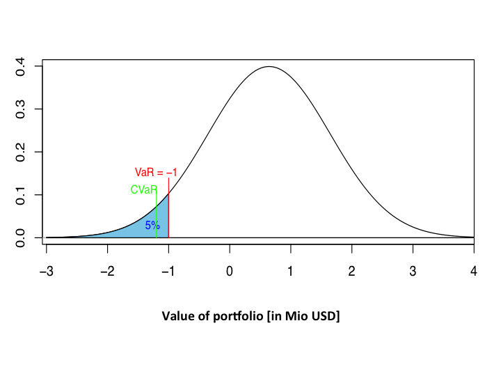
Figure 2 illustrates \(\underline{VaR}_{0.05}(Z)\), where \(Z\) is normally distributed with mean \(\mu =0.645\) and standard deviation \(\sigma = 1\).
The EMP framework provides the EMP keywords varlo and varup as a convenient alternative to chance constraints to model Value at Risk.
VaR with EMP: A Simple Example
We continue to illustrate with the stochastic portfolio model that we have already used above. Consider that the investor might be interested in a strategy that maximizes the threshold at a certain cutoff, say at 10% on the left tail of the return curve. Mathematically, the problem can be expressed as follows:
\begin{equation}\tag{41} \begin{array}{ll} \textrm{Max} & \underline{VaR}_{\theta}[R] \\ \textrm{s.t} & R = \sum_j w_j v_j\\ & \sum_j w_j = 1 \\ & w_j \geq 0,\\ \end{array} \end{equation}
where \(\underline{VaR}_{\theta}\) is the Value at Risk at the lower \(\theta\)th percentile.
In the EMP annotations of the corresponding GAMS model we introduce a new variable for VaR (varr), a scalar to specify the percentile we are interested in (theta) and the EMP keyword varlo:
* Core Model
$include data.gms
Variables
      r       "value of portfolio under each scenario"
      w(j)    "portfolio selection"
      varr    "value at risk of r"
      obj     "objective variable" ;
Positive Variables
      w ;

Scalar
      theta   "relative volume" / 0.1 /;

Equations
      defr    "return of portfolio"
      budget  "budget constraint"
      defobj  "objective equation" ;

defr..     r =e= sum(j, v(j)*w(j));
budget..   sum(j, w(j)) =e= 1;
defobj..   obj =e= varr;

Model portfolio / all /;

* EMP Annotations
File emp / '%emp.info%' /
put emp '* problem %gams.i%'
      / 'varlo r varr ' theta
      / 'stage 1 obj defobj varr'
      / 'stage 2 r defr v'
      / "jrandvar v('att') v('gmc') v('usx')"
loop(s,
  put / p(s) vs(s,"att") vs(s,"gmc") vs(s,"usx"));
putclose emp;

* Dictionary
Parameters
      s_v(s,j) "return from assets by scenario"
      s_r(s)   "return from portfolio by scenario" ;

Set   dict / s  .scenario.''
             v  .randvar .s_v
             r  .level   .s_r /;

solve portfolio using emp max obj scenario dict;
The first line in the EMP annotations begins with the EMP keyword varlo. This line specifies that the variable varr is the Value at Risk relating to the random variable r and the scalar theta is the percentile (in range 0 to 1) we consider. The other lines in the annotations are similar to the second model above. Note that the objective equals the Value at Risk at the left tail, denoted by \(\underline{VaR}\).
Observe that the EMP keyword varlo specifies VaR at the left tail of the probability distribution. For the right tail of the distribution, the EMP keyword to be used is varup.
- Note
- The keyword
varis identical tovarupwhich refers to the right tail of the distribution. - Currently only the solver DE supports the keywords for VaR.
- The keyword
Note further, that it is only appropriate to maximize \(\underline{VaR}_{\alpha}\) and minimize \(\overline{VaR_{\alpha}}\).
The implementation of the keywords varlo and varup is based on a mixed integer program similar to that described in section Example with a Single Chance Constraint. Observe that these implementations are likely to be hard and/or time consuming to solve. There is an option that allows users to customize the big \(M\) value (default is 1000) in the same manner that we outline below:
$onecho > de.opt
VaRBigM = 500
$offecho
portfolio.optfile=1;
Observe that the EMP framework offers an alternative, shorter way to model VaR. There is no additional variable for VaR, hence in the EMP annotations, the EMP keyword varlo is only followed by theta and the objective variable in the solve statement is r. As varlo is specified in the annotations, the risk measure is applied to the objective variable implicitly. The modified EMP annotations and the new solve statement follow.
File emp / '%emp.info%' /;
put emp '* problem %gams.i%'
      / 'varlo ' theta
      / 'stage 2 r defr v'
      / "jrandvar v('att') v('gmc') v('usx')"
loop(s,   put / p(s) vs(s,"att") vs(s,"gmc") vs(s,"usx"));
putclose emp;
...
solve portfolio using emp max r scenario dict;
Note that this alternative notation is shorter, but it is also opaque, therefore we recommend the first way.
Combining VaR and Expected Value
In a variation of the example above, consider an investor who aims to take into account both, the expected return and the Value at Risk of the return at a certain threshold \(\theta\). She combines the two risk measures and uses a scalar ( \(\lambda\)) as a weight. A mathematical formulation of the problem reads as follows:
\begin{equation}\tag{42} \begin{array}{ll} \textrm{Max} & \lambda \mathbb{E}[R] + (1-\lambda) \underline{VaR}_{\theta}[R] \\ \textrm{s.t} & R = \sum_j w_j v_j\\ & \sum_j w_j = 1 \\ & w_j \geq 0,\\ \end{array} \end{equation}
where \(\mathbb{E}[R]\) is the expected value of the return and \(\underline{VaR}_{\theta}\) is the Value at Risk at the \(\theta\)th percentile.
This problem can be modeled in GAMS EMP as follows:
* Core Model
$include data.gms
Variables
      r       "value of portfolio under each scenario"
      w(j)    "portfolio selection"
      varr    "value at risk of r"
      evr     "expected value of r"
      obj     "objective variable" ;
Positive Variables
      w ;

Scalars
      theta   "relative volume" / 0.1 /
      lambda  "weight EV versus VaR"  / 0.2 /;

Equations
      defr    "return of portfolio"
      budget  "budget constraint"
      defobj  "convex combination of both risk measures" ;

defr..     r =e= sum(j, v(j)*w(j));
budget..   sum(j, w(j)) =e= 1;
defobj..   obj =e= lambda*evr + (1-lambda)*varr;

Model portfolio_ext / all /;

* EMP Annotations
File emp / '%emp.info%' /
put emp '* problem %gams.i%'
      / 'ExpectedValue r evr'
      / 'varlo r varr ' theta
      / 'stage 2 r defr v'
      / 'stage 1 defobj obj'
      / "jrandvar v('att') v('gmc') v('usx')"
loop(s,
  put / p(s) vs(s,"att") vs(s,"gmc") vs(s,"usx"));
putclose emp;

* Dictionary
Parameters
      s_v(s,j) "return from assets by scenario /s1.att 1/"
      s_r(s)   "return from portfolio by scenario" ;

Set   dict / s  .scenario.''
             v  .randvar .s_v
             r  .level   .s_r /;

solve portfolio_ext using EMP max obj scenario dict;
Note that we introduced a variable for the expected value of the return like in the example above where we modeled the expected return explicitly. Note further, that we added the parameter lambda and we defined the variable obj to be the weighted sum of the expected value of the return evr and the lower VaR varr. Observe that in the EMP annotations both keywords ExpectedValue and varlo are used. The other parts of the model remain unchanged.
Conditional Value at Risk (CVaR)
The Conditional Value at Risk (CVaR) is the expected value of the left or right tail of the distribution; for example, the expected value of the left 5% of the standard Normal distribution. Note that CVaR is also called expected shortfall. In this subsection we introduce and discuss CVaR in more detail by presenting a mathematical formulation, demonstrating how CVaR can be modeled with GAMS EMP using a simple example and showing how to optimize the weighted sum of the expected value and CVaR.
CVaR: Mathematical Formulation
\(\underline{CVaR}_{\alpha}\) is the expected average return (in a given time period) given that we are in the \((\alpha \times 100)\)% left tail of the return distribution, where \(\alpha \in (0,1)\). In other words, \(\underline{CVaR}_{\alpha}\) is a mean of the left tail. For example, if we are interested in the 5% worst cases, i.e. \(\alpha = 0.05\), \(\underline{CVaR}_{\alpha}\) is the conditional expectation of the return, given the return is no greater than VaR.
Let \(\xi\) be a random variable with probability density function \(p(\xi)\), let \(G(\xi)\) be a function of the random variable \(\xi\) denoting the return of a portfolio of assets and let \(\alpha \in (0,1)\) be a probability. Then the conditional value at risk of \(G(\xi)\) is defined as
\begin{equation}\tag{43} \underline{CVaR}_{\alpha}(G(\xi)) = \frac{1}{\alpha} \int_{-\infty}^{VaR_{\alpha}} G(\xi) \cdot p(\xi) d\xi, \end{equation}
where \(VaR_{\alpha}\) is the value at risk.
CVaR with EMP: A Simple Example
In the stochastic portfolio example that we have used throughout this section, the investor might be interested to make sure that in the worst cases she loses as little as possible. Thus she could consider only the worst 10% of possible cases and allocate her funds such that the expected mean return in these cases is maximized. Mathematically, the problem can be expressed as follows:
\begin{equation}\tag{44} \begin{array}{ll} \textrm{Max} & \underline{CVaR}_{\theta}[R] \\ \textrm{s.t} & R = \sum_j w_j v_j\\ & \sum_j w_j = 1 \\ & w_j \geq 0,\\ \end{array} \end{equation}
where \(\underline{CVaR}_{\theta}\) is the CVaR at the confidence level \(\theta\) at the left tail of the distribution.
Like in the case of Value at Risk above, we introduce a new variable for CVaR (cvarr), a scalar to specify the percentile we are interested in (theta) and the EMP keyword cvarlo in the EMP annotations:
* Core Model
$include data.gms
Variables
      r       "value of portfolio under each scenario"
      w(j)    "portfolio selection"
      cvarr   "conditional value at risk of r"
      obj     "objective variable" ;
Positive Variables
      w ;

Scalar
      theta   "relative volume" / 0.1 /;

Equations
      defr    "return of portfolio"
      budget  "budget constraint"
      defobj  "objective equation" ;

defr..     r =e= sum(j, v(j)*w(j));
budget..   sum(j, w(j)) =e= 1;
defobj..   obj =e= cvarr;

Model portfolio / all /;

* EMP Annotations
File emp / '%emp.info%' /
put emp '* problem %gams.i%'
      / 'cvarlo r cvarr' theta
      / 'stage 1 obj defobj cvarr'
      / 'stage 2 r defr v'
      / "jrandvar v('att') v('gmc') v('usx')"
loop(s,
  put / p(s) vs(s,"att") vs(s,"gmc") vs(s,"usx"));
putclose emp;

* Dictionary
Parameters
      s_v(s,j) "return from assets by scenario"
      s_r(s)   "return from portfolio by scenario" ;

Set   dict / s  .scenario.''
             v  .randvar .s_v
             r  .level   .s_r /;

solve portfolio using emp max obj scenario dict;
In the EMP annotations, the first line starts with the EMP keyword cvarlo. This line specifies that the variable cvarr is the left-tail CVaR relating to the random variable r and the scalar theta is the fraction (in range 0 to 1) we consider. Like in the previous section, the objective variable, the objective equation and the variable in the objective equation belong to the first stage while the equation that handles the random data and all its variables belong to the second stage. Observe that the objective equals the Conditional Value at Risk.
Note that the keyword cvarlo specifies CVaR at the left tail of the probability distribution. For the right tail of the distribution the keyword to be used is cvarup.
- Note
- The EMP keyword
cvaris identical to the keywordcvarup. - Currently only the solver DE supports the keywords for CVaR.
- The EMP keyword
The conditional value at risk denoting the mean of the right tail of the distribution can be denoted by \(\overline{CVaR}\) and is defined as:
\begin{equation}\tag{45} \overline{CVaR}_{\alpha}(G(\xi)) = \frac{1}{1-\alpha} \int_{VaR_{\alpha}}^{\infty} G(\xi) \cdot p(\xi) d\xi. \end{equation}
Observe that it is only appropriate to maximize \(\underline{CVaR}_{\alpha}\) and minimize \(\overline{CVaR_{\alpha}}\). Furthermore, \(\underline{CVaR}_{\alpha}\) is a concave function and so should only be constrained using e.g.
\[ \underline{CVaR}_{\alpha} \geq \gamma \]
and \(\overline{CVaR_{\alpha}}\) is convex, so should only appear in constraints like
\[ \overline{CVaR_{\alpha}} \leq \gamma. \]
The EMP framework offers an alternative way to model CVaR. In this alternative formulation, there is no additional variable for CVaR, hence in the EMP annotations, the EMP keyword cvarlo is only followed by theta and the objective variable in the solve statement is r. As cvarlo is specified in the annotations, the risk measure is applied to the objective variable implicitly. The modified EMP annotations and the new solve statement follow.
File emp / '%emp.info%' /
put emp '* problem %gams.i%'
      / 'cvarlo ' theta
      / 'stage 2 r defr v'
      / "jrandvar v('att') v('gmc') v('usx')"
loop(s,   put / p(s) vs(s,"att") vs(s,"gmc") vs(s,"usx"));
putclose emp;
...
solve portfolio using emp max r scenario dict;
Note that this alternative notation is shorter, but it is considerably less clear, therefore we recommend the explicit notation of the first model.
Combining CVaR and Expected Value
In a final variation on the portfolio example, we consider an investor who aims to take into account both, the expected return and the Conditional Value at Risk of the return at a certain threshold \(\theta\). She combines the two risk measures and uses a scalar ( \(\lambda\)) to weigh the two summands. A mathematical formulation of the problem reads as follows:
\begin{equation}\tag{46} \begin{array}{ll} \textrm{Max} & \lambda \mathbb{E}[R] + (1-\lambda) \underline{CVaR}_{\theta}[R] \\ \textrm{s.t} & R = \sum_j w_j v_j\\ & \sum_j w_j = 1 \\ & w_j \geq 0,\\ \end{array} \end{equation}
where \(\mathbb{E}[R]\) is the expected value of the return and \(\underline{CVaR}_{\theta}\) is the CVaR at the confidence level \(\theta\).
This problem can be modeled with GAMS EMP as follows:
* Core Model
$include data.gms
Variables
      r       "value of portfolio under each scenario"
      w(j)    "portfolio selection"
      cvarr   "conditional value at risk of r"
      evr     "expected value of r"
      obj     "objective variable" ;
Positive Variables
      w ;

Scalars
      theta   "relative volume" / 0.1 /
      lambda  "weight EV versus CVaR"  / 0.2 /;

Equations
      defr    "return of portfolio"
      budget  "budget constraint"
      defobj  "convex combination of both risk measures" ;

defr..     r =e= sum(j, v(j)*w(j));
budget..   sum(j, w(j)) =e= 1;
defobj..   obj =e= lambda*evr + (1-lambda)*cvarr;

Model portfolio_ext / all /;

* EMP Annotations
File emp / '%emp.info%' /
put emp '* problem %gams.i%'
      / 'ExpectedValue r evr'
      / 'cvarlo r cvarr ' theta
      / 'stage 2 r defr v'
      / 'stage 1 defobj obj'
      / "jrandvar v('att') v('gmc') v('usx')"
loop(s,
  put / p(s) vs(s,"att") vs(s,"gmc") vs(s,"usx"));
putclose emp;

* Dictionary
Parameters
      s_v(s,j) "return from assets by scenario"
      s_r(s)   "return from portfolio by scenario" ;

Set   dict / s  .scenario.''
             v  .randvar .s_v
             r  .level   .s_r /;

solve portfolio_ext using emp max obj scenario dict;
Note that apart from the EMP keyword varlo being replaced by cvarlo, the code is identical to the code above, where we maximized the weighted sum of the expected value and VaR. Observe that by decreasing the value of \(\lambda\) from 1 to 0 we can explore the results of an increasingly risk averse behavior.
EMP Syntax for Risk Measures
The EMP annotations where risk measures are used have the same general syntax like stochastic models with recourse. In addition, the following keywords may be used:
ExpectedValue rv var
varlo [rv var] scalar
varup [rv var] scalar
cvarlo [rv var] scalar
cvarup [rv var] scalar
The EMP keyword Expected Value is used to state that the variable var is the expected value of the random variable rv. Note that the random variable rv must be defined to be a random variable in the EMP annotations.
The EMP keywords varlo, varup, cvarlo and cvarup refer to VaR at the left tail of the distribution ( \(\underline{VaR}_{\alpha}\)), VaR at the right tail of the distribution ( \(\overline{VaR}_{\alpha}\)), CVaR at the left tail of the distribution ( \(\underline{CVaR}_{\alpha}\)) and CVaR at the right tail of the distribution ( \(\overline{CVaR}_{\alpha}\)) respectively.
- Note
- The EMP keyword
varis a synonym tovarupandcvaris a synonym tocvarup.
The specifications that follow all four keywords have a long and a short version. In the long version, the random variable rv and the variable that is assigned to be the respective risk measure (VaR or CVaR) are named explicitly. The scalar is a number in the interval \((0,1)\), it defines the percentile in VaR and confidence level in CVaR. In the short version, only the scalar is specified. In this case the risk measure will applied to the objective variable implicitly.
- Note
- These five keywords are only supported by the solver DE.
Chance Constraints with EMP
In stochastic programs with chance constraints the goal is to make an optimal decision prior to the realization of random data while allowing the constraints (or some of them) to be violated with a certain probability. Note that chance constraints are also called probabilistic constraints.
This section is organized as follows. After introducing a mathematical formulation of chance constraints, we show how such problems can be modeled with GAMS EMP using a simple example with only one chance constraint. Then we extend the model to include multiple chance constraints. We discuss the two ways to model problems with multiple chance constraints: using joint chance constraints and using individual chance constraints. Joint chance constraints require that all constraints are satisfied simultaneously with a given probability. Individual chance constraints require each constraint to be satisfied with a given probability independently of other constraints. Further, the EMP framework offers the option to penalize the violation of chance constraints. This is the topic of subsection Penalizing Violations of Chance Constraints. We conclude this section with an overview of the EMP annotations that are specific to chance constraints.
Chance Constraints: Mathematical Formulation
Mathematically, a stochastic linear program with chance constraints can be expressed as follows:
\begin{equation}\tag{47} \begin{array}{ll} \textrm{Min}_{x} & c^T x \\ \textrm{s.t.} & P(A x \leq b) \geq p\\ & x \geq 0,\\ \end{array} \end{equation}
where \( x \in \mathbb{R}^n \) is the decision variable and \( c^T \) denotes the coefficients of the objective function, \( A \in \mathbb{R}^{m \times n} \) is a random matrix and represents the coefficients and \( b \in \mathbb{R}^m \) is a random vector and denotes the right-hand side of the constraints. The distinctive feature of stochastic programs with chance constraints is that the constraints (or some of them) may be violated with probability \( \epsilon = 1-p \), where \(0 < p \leq 1\). Note that \( \epsilon \) is sometimes called the risk tolerance.
One way to solve a stochastic problem with chance constraints is to convert it to a mixed-integer problem (MIP) first and then solve the MIP equivalent. The idea is to introduce a set of scenarios \(S\) and a vector with binary variables, say \(y_k \in \mathbb{R}^m\), for each scenario \(k \in S\). The binary variables take value 1 if the corresponding constraint is satisfied in a scenario and 0 otherwise. A scenario-based formulation of the chance-constrained stochastic linear program above can be written as:
\begin{equation} \tag{48} \begin{array}{ll} \textrm{Min}_{x} & c^T x \\ \textrm{s.t.} & A^k x \leq b^k + M^k(1-y_k)\\ & \sum_{k \in S} y_k \geq p \times |S|\\ & x \geq 0, \quad y \in (0,1)^{|S|},\\ \end{array} \end{equation}
where \(M^k \in \mathbb{R}^m\) is a chosen big-M vector. The entries of the vector \(M^k\) should be chosen such that it does not cut off any feasible solution if \(y_k = 0\).
Example with a Single Chance Constraint
We start with the simplest case, where the random matrix \(A\) consists of just one random vector \(a\), resulting in a problem with a single chance constraint. The following example is adapted from model [SIMPLECHANCE].
\begin{equation} \tag{49} \begin{array}{lll} \textrm{Min} & x_1 + x_2 \\ \textrm{s.t.} & P(\omega x_1 + x_2 \geq 7) \geq 0.75, &\quad \omega \in \Omega = \{1, 2, 3, 4\}\\ & x_1, x_2 \geq 0. \end{array} \end{equation}
Here the random parameter \(\omega\) has four possible realizations. Thus we have four scenarios and we assume that each scenario is equally likely to be realized, i.e. \(\pi^k = \frac{1}{4}\), where \(\pi^k\) denotes the probability that scenario \(k\) is realized. Note that in this example \(b\) is fixed at 7. As \(p=0.75\) and each scenario is equally likely to be realized, we need to choose \(x_1\) and \(x_2\) such that the inequality is satisfied in at least 3 scenarios. For clarity, we spell out the inequalities for the scenarios:
\begin{equation} \tag{50} \begin{array}{lll} k=1: & \omega_1 = 1 & \omega_1 x_1 + x_2 \geq 7 \\ k=2: & \omega_2 = 2 & \omega_2 x_1 + x_2 \geq 7 \\ k=3: & \omega_3 = 3 & \omega_3 x_1 + x_2 \geq 7 \\ k=4: & \omega_4 = 4 & \omega_4 x_1 + x_2 \geq 7. \\ \end{array} \end{equation}
The MIP equivalent of problem (49) is given below:
\begin{equation} \tag{51} \begin{array}{lll} \textrm{Min} & x_1 + x_2 \\ \textrm{s.t.} & 1 x_1 + x_2 \geq 7 - M (1-y_1)\\ & 2 x_1 + x_2 \geq 7 - M (1-y_2)\\ & 3 x_1 + x_2 \geq 7- M (1-y_3) \\ & 4 x_1 + x_2 \geq 7 - M (1-y_4)\\ \\ & cc_1 = 1 - \sum_k \pi^k y_k, \quad k=1, \dots, 4, \, \pi^k = \frac{1}{4}\\ \\ & x_1, x_2 \geq 0 \\ & 0 \leq cc_1 \leq (1 - 0.75) \\ & y_k \in (0,1). \end{array} \end{equation}
Observe that the first four constraints cover the four possible scenarios with \(\omega\) taking the values 1, 2, 3 and 4 respectively. On the right-hand side we introduce a big-M factor and \(y_k\), a binary indicator variable. \(y_k\) takes the value 1 if the constraint is satisfied and zero otherwise. The new variable \(cc_1\) represents the probability that the constraint is violated. If \(cc_1\) equals zero, the sum will equal 1, indicating that the constraint is satisfied in all four scenarios. If \(cc_1 = 0.25\), the constraint will be unsatisfied in one scenario out of four (for this scenario \(y_k =0\)).
The problem can be modeled in GAMS EMP as follows:
* Core Model
Positive Variables x1, x2;
Variables          z;

Scalar om  / 1 /;

Equations obj, e1;

obj..   z =e= x1 + x2;
e1..    om*x1 + x2 =g=  7;

Model sc / all /;

* EMP Annotations
File emp / '%emp.info%' /;
put emp;
$onput
randvar om discrete 0.25 1  0.25 2   0.25 3   0.25 4
chance e1 0.75
$offput
putclose emp;

* Dictionary
Set scen "scenarios" / s1*s4 /;
Parameter  s_om(scen)
       x1_l (scen)
       x2_l (scen)
       e1_l (scen);

Set dict / scen .scenario.''
            om  .randvar .s_om
            x1  .level   .x1_l
            x2  .level   .x2_l
            e1  .level   .e1_l/;

solve sc min z use EMP scenario dict;
display s_om, x1_l, x2_l, e1_l;
Like other EMP stochastic programming models, the model consists of three parts: the core model, the EMP annotations and the dictionary with output-handling information. As usual, the core model is defined as a deterministic model and the specifications relating to the stochastic structure of the problem are written to the file emp.info. In the EMP annotations, the EMP keyword randvar is used to declare a parameter from the core model as a random variable. The keyword is followed by om, the random variable, and the distribution. The EMP keyword discrete indicates that we have a discrete distribution. The discrete distribution is specified via probability-numerical value pairs. Note that continuous distributions are also possible. See section Random Variables with Continuous Distributions for more information. The second line in the EMP annotations starts with the EMP keyword chance followed by the equation e1 and a probability. The specification means that the constraints e1 must hold for at least 75% of all scenarios. We can verify that this requirement has been enforced by checking in the listing file the level value of the constraint e1_l. We will see that in the first scenario the constraint was violated, but is was satisfied in all other scenarios.
Observe that the EMP keyword chance allows for an optional specification that is related to a penalization factor for constraints that are violated. This topic is discussed in section Penalizing Violations of Chance Constraints below.
- Note
- Currently, there are no stages in stochastic problems with chance constraints, unlike in stochastic problems with recourse.
As the problem is solved as a MIP, it is important that the options OptCA and OptCR are assigned appropriate values.
Note that the default value of \(M\) is 1e7 for the solver Lindo. To customize this and set it to, e.g., 1000 instead, one could insert the following five lines before the solve statement:
option emp = lindo;
$onecho > lindo.opt
STOC_BIGM 1e3
$offecho
sc.optfile = 1;
For DE the default value of \(M\) is 10000 and it could be changed to 1000 in a similar way as seen above for Lindo:
option emp = de;
$onecho > de.opt
ccreform bigM 1e3
$offecho
sc.optfile = 1;
Note that ccreform is a DE option. This option allows to specify two alternative solution strategies: a reformulation using a convex hull and a reformulation using indicator variables and indicator constraints. The following line indicates that a convex hull with \(M = 1000\) and \(\epsilon = 0.00001\) is to be used:
ccreform cHull 1e3 1e-6
For indicator variables and constraints, the following line is used:
ccreform indic
Note that currently only the solver CPLEX supports indicator variables, so the resulting reformulated problem has to be solved with CPLEX.
Examples with Multiple Chance Constraints
Stochastic problems with multiple chance constraints have two different forms: problems with joint chance constraints and problems with multiple individual chance constraints. In problems with joint chance constraints the constraints all have to be satisfied simultaneously with probability \(p\). In problems with multiple individual chance constraints each constraint carries its own risk tolerance. We illustrate with two examples.
Joint Chance Constraints
We illustrate joint chance constraints by extending the example above by one constraint resulting in a problem with two chance constraints:
\begin{equation} \tag{52} \begin{array}{lll} \textrm{Min} & x_1 + x_2 \\ \textrm{s.t.} & P(\omega_1 x_1 + x_2 \geq 7; \, \, \omega_2 x_1 + 3 x_2 \geq 12) \geq 0.6, &\quad (\omega_1,\omega_2) \in \Omega \\ & x_1, x_2 \geq 0, \end{array} \end{equation}
where
\begin{equation} \Omega = \{ (1,1), (1,2), (1,3), (2,1), (2,2), (2,3), (3,1), (3,2), (3,3), (4,1), (4,2), (4,3) \} \end{equation}
and
\begin{equation} \pi^k = \pi(\omega_1, \omega_2) = \frac{1}{12} \quad \textrm{for all} \quad (\omega_1, \omega_2) \in \Omega. \end{equation}
Note that both random variables follow discrete uniform distributions, \(\omega_1\) has four realizations and \(\omega_2\) has three realizations. Thus we have 12 scenarios that are all equally likely. The MIP equivalent takes the following form:
\begin{equation} \tag{53} \begin{array}{lll} \textrm{Min} & x_1 + x_2 \\ \\ \textrm{s.t.} & 1 x_1 + x_2 \geq 7 - M (1-y_1)\\ & 1 x_1 + 3 x_2 \geq 12 - M (1-y_1)\\ & 2 x_1 + x_2 \geq 7 - M (1-y_2)\\ & 1 x_1 + 3 x_2 \geq 12 - M (1-y_2)\\ & \vdots \\ & 4 x_1 + x_2 \geq 7 - M (1-y_{12})\\ & 3 x_1 + 3 x_2 \geq 12 - M (1-y_{12})\\ \\ & cc_1 = 1 - \sum_k \pi^k y_k, \quad k=1, \dots, 12, \, \pi^k = \frac{1}{12}\\ & x_1, x_2 \geq 0 \\ & 0 \leq cc_1 \leq (1 - 0.6) \\ & y_k \in (0,1). \end{array} \end{equation}
Note that the first set of constraints covers the 12 scenarios, where each scenario has two constraints. The other constraints are similar to those introduced in the previous model.
The problem can be modeled with GAMS EMP as follows:
* Core Model
Positive Variables x1, x2;
Variables          z;

Scalars om1, om2;
om1 = 1;
om2 = 1;

Equations obj, e1, e2;

obj..   z =e= x1 + x2;
e1..    om1*x1 +   x2 =g=  7;
e2..    om2*x1 + 3*x2 =g= 12;

Model sc / all /;

* EMP Annotations
File emp / '%emp.info%' /;
put emp '* problem %gams.i%'/;
$onput
randvar om1 discrete 0.25 1  0.25 2  0.25 3  0.25 4
randvar om2 discrete 0.3333 1  0.3334 2  0.3333 3
chance e1 e2 0.6
$offput
putclose emp;

* Dictionary
Set scen "scenarios" / s1*s12 /;
Parameters  s_om1(scen)
            s_om2(scen)
            x1_l (scen)
            x2_l (scen)
            e1_l (scen)
            e2_l (scen);

Set dict / scen .scenario.''
           om1  .randvar .s_om1
           om2  .randvar .s_om2
           x1   .level   .x1_l
           x2   .level   .x2_l
           e1   .level   .e1_l
           e2   .level   .e2_l/;

solve sc min z use emp scenario dict;
display s_om1, s_om2, x1_l, x2_l, e1_l, e2_l;
In the EMP annotations, the line chance e1 e2 0.6 specifies that in at least 60% of all scenarios both constraints e1 and e2 must be satisfied at the same time. There are a total of 12 scenarios, hence both constraints must be satisfied in at least 8 scenarios (i.e. \(12 \times 0.6=7.2 \leq 8\)). We can verify that this requirement has been enforced by checking in the listing file the level values of the constraints, e1_l and e2_l. Indeed, in the optimal solution both constraints hold in scenarios 4 to 12, meaning that there are 9 scenarios that satisfy both inequalities.
Individual Chance Constraints
In stochastic problems with individual chance constraints there is no correlation between the probabilities of the rows of the matrix \(A\). Hence problem (47) takes the following form:
\begin{equation} \tag{54} \begin{array}{ll} \textrm{Min}_{x} & c^T x \\ \textrm{s.t.} & P(A_i x \leq b_{i}) \geq p_i, \quad i=1, \dots, m\\ & x \geq 0.\\ \end{array} \end{equation}
To illustrate, we use an extended version of the the example from the previous section and replace the joint chance constraints by individual chance constraints:
\begin{equation} \tag{55} \begin{array}{lll} \textrm{Min} & x_1 + x_2 \\ \textrm{s.t.} & P(\omega_1 x_1 + x_2 \geq 7) \geq 0.75, &\quad \omega_1 \in \Omega _1 = \{1, 2, 3, 4\}\\ & P(\omega_2 x_1 + 3 x_2 \geq 12) \geq 0.6, & \quad \omega_2 \in \Omega _2 = \{1, 2, 3\} \\ &P(\omega_1 x_1 + \omega_2 x_2 \geq 10) \geq 0.5, & \quad (\omega_1, \omega_2) \in \Omega_1 \times \Omega_2 = \Omega\\ & x_1, x_2 \geq 0. \end{array} \end{equation}
Note that \(\Omega\) is defined as in (52) above, we have again 12 scenarios, each with probability \(\pi^k = \frac{1}{12}\). However, in this example, the first inequality must hold in 9 out of 12 scenarios ( \(0.75 \times 12=9\)), the second inequality must hold in 8 out of 12 inequalities ( \(0.6\times 12=7.2 \leq 8\)) and the third inequality must hold in 6 out of 12 scenarios. Note further, that we may have four types of scenarios: scenarios where all constraints are violated, scenarios where two constraints are violated, scenarios where one constraint is violated and scenarios where all three constraints are satisfied. The only condition is that for each constraint there is the respective number of scenarios where the constraint is satisfied. Observe that the random data in the third inequality is a combination of the random data of the first two inequalities. The inequalities for the scenarios are given below:
\begin{equation} \tag{56} \begin{array}{lll} k=1: & \omega_{1}^{1} = 1, \, \, \omega_{2}^{1} = 1 & \omega_{1}^{1} x_1 + x_2 \geq 7\\ & &\omega_{2}^{1} x_1 + 3 x_2 \geq 12 \\ & & \omega_{1}^{1} x_1 + \omega_{2}^{1} x_2 \geq 10\\ k=2: & \omega_{1}^{2} = 1, \, \, \omega_{2}^{2} = 2 & \omega_{1}^{2} x_1 + x_2 \geq 7\\ & & \omega_{2}^{2} x_1 + 3 x_2 \geq 12\\ & & \omega_{1}^{2} x_1 + \omega_{2}^{2} x_2 \geq 10\\ \vdots\\ k=12: & \omega_{1}^{12} = 4, \, \, \omega_{2}^{12} = 3 & \omega_{1}^{12} x_1 + x_2 \geq 7\\ & & \omega_{2}^{12} x_1 + 3 x_2 \geq 12\\ & & \omega_{1}^{12} x_1 + \omega_{2}^{12} x_2 \geq 10\\ \end{array} \end{equation}
The MIP equivalent follows:
\begin{equation} \tag{57} \begin{array}{lll} \textrm{Min} & x_1 + x_2 \\ \\ \textrm{s.t.} & 1 x_1 + x_2 \geq 7 - M (1-y^{1}_{1})\\ & 1 x_1 + 3 x_2 \geq 12 - M (1-y^{2}_{1})\\ & 1 x_1 + 1 x_2 \geq 10 - M (1-y^{3}_{1})\\ & 2 x_1 + x_2 \geq 7 - M (1-y^{1}_{2})\\ & 1 x_1 + 3 x_2 \geq 12 - M (1-y^{2}_{2})\\ & 2 x_1 + 1 x_2 \geq 10 - M (1-y^{3}_{2})\\ & \vdots \\ & 4 x_1 + x_2 \geq 7 - M (1-y^{1}_{12})\\ & 3 x_1 + 3 x_2 \geq 12 - M (1-y^{2}_{12})\\ & 4 x_1 + 3 x_2 \geq 10 - M (1-y^{3}_{12})\\ \\ & cc_1 = 1 - \sum_k \pi^k y^{1}_{k}, \quad k=1, \dots, 12, \quad \pi^k = \frac{1}{12}\\ & cc_2 = 1 - \sum_k \pi^k y^{2}_{k}, \quad k=1, \dots, 12, \quad \pi^k = \frac{1}{12}\\ & cc_3 = 1 - \sum_k \pi^k y^{3}_{k}, \quad k=1, \dots, 12, \quad \pi^k = \frac{1}{12}\\ \\ & x_1, x_2 \geq 0 \\ & 0 \leq cc_1 \leq (1 - 0.75) \\ & 0 \leq cc_2 \leq (1 - 0.6) \\ & 0 \leq cc_3 \leq (1 - 0.5) \\ & y^{j}_{k} \in (0,1). \end{array} \end{equation}
As expected, there are three constraints for every scenario. Note that we introduced three new variables, \(cc_1\), \(cc_2\) and \(cc_3\) and three corresponding constraints. Each of the variables has a different range reflecting the different probabilities with which a constraint may be violated.
The core model of the GAMS code is very similar to the core model with joint chance constraints. We just add the third inequality:
Equations obj, e1, e2, e3;

obj..   z =e= x1 + x2;
e1..    om1*x1 +   x2 =g=  7;
e2..    om2*x1 + 3*x2 =g= 12;
e3..    om1*x1 + om2*x2 =g= 10;
There is a slight modification in the annotations:
File emp / '%emp.info%' /;
put emp '* problem %gams.i%'/;
$onput
randvar om1 discrete 0.25 1   0.25 2  0.25 3  0.25 4
randvar om2 discrete 0.3333 1  0.3334 2  0.3333 3
chance e1 0.75
chance e2 0.6
chance e3 0.5
$offput
putclose emp;
Observe that we have three lines that start with the EMP keyword chance: every constraint is listed separately with its respective probability.
- Note
- In case one constraint has to be satisfied in all scenarios (so it is strictly speaking not a chance constraint), then it has to be listed with probability 1.0.
An overview of which constraints are satisfied in which scenarios in the optimal solution is given in the following table:
| Scenarios | 1 | 2 | 3 | 4 | 5 | 6 | 7 | 8 | 9 | 10 | 11 | 12 |
|---|---|---|---|---|---|---|---|---|---|---|---|---|
Scenarios where e1 is satisfied | x | x | x | x | x | x | x | x | x | |||
Scenarios where e1 is satisfied | x | x | x | x | x | x | x | x | ||||
Scenarios where e1 is satisfied | x | x | x | x | x | x | x |
Table 7: Overview of constraint satisfaction per scenario
Observe that all constraints are satisfied in as many scenarios as required and there are scenarios where all three constraints are satisfied ( \(k = 6, 8, 9, 11, 12\)), scenarios where only two constraints are satisfied ( \(k = 5, 7, 10\)), scenarios where only one constraint is satisfied ( \(k = 2, 3, 4\)) and one scenario where all constraints are violated ( \(k = 1\)).
The choice whether joint or individual chance constraints should be used depends on the system being modeled. Both approaches have their own advantages. Individual chance constraints are weaker since not all constraints have to be satisfied at the same time. This can be clearly observed in the optimal solution for example (55). The objective value is 5.20 in the model with joint chance constraints and 4.75 in the model with individual chance constraints (assuming that each constraint is satisfied in 60% of all scenarios). As it is a minimizing problem, the model with individual chance constraints yields the better result. However, in this solution we have only 6 scenarios where both constraints are simultaneously satisfied while each constraint is satisfied in eight scenarios in total for the joint chance constraint formulation, as required.
Penalizing Violations of Chance Constraints
The EMP framework provides the syntax for a penalty factor for each scenario that violates one or more constraints. In the example with joint constraints above, the EMP annotations could be modified in the following way:
$onput
randvar om1 discrete 0.25 1  0.25 2  0.25 3  0.25 4
randvar om2 discrete 0.3333 1  0.3334 2  0.3333 3
chance e1 e2 0.6 3
$offput
Note that we added the number 3 at the end of the last line. This new entry represents a penalty factor. Recall that the MIP equivalent (53 ) takes the following form:
\begin{equation} \tag{58} \begin{array}{lll} \textrm{Min} & z = x_1 + x_2 \\ \textrm{s.t.} & 1 x_1 + x_2 \geq 7 - M (1-y_1)\\ & 1 x_1 + 3 x_2 \geq 12 - M (1-y_1)\\ & \vdots \\ & 4 x_1 + x_2 \geq 7 - M (1-y_{12})\\ & 3 x_1 + 3 x_2 \geq 12 - M (1-y_{12})\\ & cc_1 = 1 - \sum_k \pi^k y_k, \quad k=1, \dots, 12, \quad \pi^k = \frac{1}{12}\\ & x_1, x_2 \geq 0 \\ & 0 \leq cc_1 \leq (1 - 0.6) \\ & y_k \in (0,1). \end{array} \end{equation}
Observe that the probability with which the constraints are allowed to be violated is stored in the variable \(cc_1\). Introducing a penalty factor or weight \(w\) has the effect that the term \( (w \times cc_1) \) is added to the objective function:
\begin{equation} z = x_1 + x_2 + w \times cc_1 = x_1 + x_2 + 3 \, cc_1 \end{equation}
Similarly, we could add weights in the example with individual chance constraints:
chance E1 0.75 5
chance E2 0.6 6
chance E3 0.5 7
Given these annotations, we obtain the following objective function in the MIP equivalent:
\begin{equation} z = x_1 + x_2 + 5 \, cc_1 + 6 \, cc_2 + 7 \, cc_3. \end{equation}
Penalty terms can be useful to explore sensitivities to slight changes.
- Note
- Like in the context of soft constraints, the penalty term is added in minimization problems and subtracted in maximization problems.
Moreover, the probability expression \(cc_1\) in the MIP equivalent may be used as a variable in the original model. For example, in the joint chance constraints problem above, we could introduce a new variable, \(viol\), in the objective function:
\begin{equation} \textrm{Min} \quad z = x_1 + x_2 + 3*viol \end{equation}
Then we write the chance constraint specification in the EMP annotations as follows:
chance E1 E2 0.6 viol
The addition of the variable viol as penalty factor causes \(cc_1\) to be replaced by \(viol\) in the MIP equivalent. Thus we have:
\begin{equation} viol = 1 - \sum_k \pi^k y_k, \quad k=1, \dots, 12, \quad \pi^k = \frac{1}{12}, \quad viol \in [0, 0.4]. \end{equation}
Note that the corresponding model is equivalent to the joint chance constraints model with penalty factor 3 with which we started this subsection.
EMP Syntax for Chance Constraints
The general syntax of the EMP annotations used to specify stochastic problems with chance constraints is as follows:
[randvar rv discrete prob val {prob val}]
[randvar rv distr par {par}]
[jrandvar rv rv {rv} prob val val {val} {prob val val {val}}]
chance equ {equ} [holds] minRatio [weight|var]
{chance equ {equ} [holds] minRatio [weight|var]}
The first three lines present three ways to specify random variables. The syntax and logic is the same as in stochastic problems with recourse, see above for details. Note that at least one random variable has to be specified. The EMP keyword chance is used to define the constraint(s) that only have to hold for a certain ratio of the possible outcomes. This ratio is given with the number minRatio ( \( 0 \le \textrm{minRatio} \le 1\)). The keyword holds is optional and does not affect the solver. The remaining specifications are optional and relate to the penalization of chance constraints that are violated. If weight is defined, the violation of a chance constraint will be penalized in the objective function ( \( \textrm{weight} \times \textrm{violationRatio} \)). Alternatively, if the name of a variable of the model (var) is specified, the violation will be multiplied by the value of this variable instead of the fixed multiplier weight.
In this section we have introduced various versions of problems with chance constraints with simple examples. For a more complex example, see the farming model [KILOSAFARM] in the GAMS EMP Model Library.