Table of Contents
This research was supported by the GAMS Applied General Equilibrium Research Fund. The author remains responsible for any bugs which exist in this software.
- Date
- 1995
An Overview
This document describes a mathematical programming system for general equilibrium analysis named MPSGE which operates as a subsystem to the mathematical programming language GAMS. MPSGE is library of function and Jacobian evaluation routines which facilitates the formulation and analysis of AGE models. MPSGE simplifies the modeling process and makes AGE modeling accessible to any economist who is interested in the application of these models. In addition to solving specific modeling problems, the system serves a didactic role as a structured framework in which to think about general equilibrium systems.
MPSGE separates the tasks of model formulation and model solution, thereby freeing model builders from the tedious task of writing model-specific function evaluation subroutines. All features of a particular model are communicated to GAMS/MPSGE through a tabular input format. To use MPSGE, a user must learn the syntax and conventions of this model definition language.
The present paper is intended for students who have completed two semesters of study in microeconomics. The purpose of this presentation is to give students a practical perspective on microeconomic theory. The diligent student who works through all of the examples provided here should be capable of building small models "from scratch" to illustrate basic theory. This is a first step to acquiring a set of useable tools for applied work.
The remainder of this paper is organized as follows. Section The Theory of Consumer Demand review the theory of consumer demand; section Getting Started provides guidance on how to verify that the GAMS/MPSGE software is operational; section Modeling Consumer Demand introduces the modeling framework with three models illustrating the representation of consumer demand within the MPSGE language. Section The Pure Exchange Model reviews the pure exchange model, and section Modeling Pure Exchange with MPSGE presents two MPSGE models of exchange. Each of the model- oriented sections present exercises based on the models which give students a chance to work through the material on their own. Additional introductory examples for self-study can be found in the Markusen library as well as in the GAMS Model Library (look for models with names ending in "MGE").
The level of presentation and diagrammatic exposition adopted here is based on Hal Varian's undergraduate microeconomics textbook ( Intermediate Microeconomics: A Modern Approach, Third Edition, W. W. Norton & Company, Inc., 1993).
The ultimate objective of this piece is to remind students of some theory which they have already seen and illustrate how these ideas can be used to build numerical models using GAMS with MPSGE. It is not my intention to provide a graduate level presentation of this material. So far as possible, I have avoided calculus and even algebra. The objective here is to demonstrate that what matters are economic ideas. With the proper tools, it is possible to do concrete economic modeling without a lot of mathematical formalism.
The Theory of Consumer Demand
A central idea underlying most microeconomic theory is that agents optimize subject to constraints. The optimizing principle applied to consumer choice begins from the notion that agents have preferences over consumption bundles and will always choose the most preferred bundle subject to applicable constraints. To operationalize this theory, three issues which must be addressed:
- How can we represent preferences?
- What is the nature of constraints on consumer choice? and
- How can the choice be modelled?
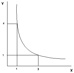
Preferences are relationships between alternative consumption "bundles". These can be represented graphically using "indifference
curves", as illustrated in Figure 1. Focusing now on the preferences of a single consumer, the indifference curve is a line which connects all combinations of two goods x and y between which our consumer is indifferent. As this curve is drawn, we have represented an agent with "well-behaved preferences": at any allocation, more is better (monotonicity), and averages are preferred to extremes (convexity). Exactly one such indifference curve goes through each positive combination of x and y. Higher indifference curves lie to the "north-east".
If we wish to characterize an agent's preferences, the "marginal rate of
substitution" (MRS) is a useful point of reference. At a given combination of x and y, the marginal rate of substitution is the slope of the associated indifference curve. As drawn, the MRS increases in magnitude as we move to the northwest and the MRS decreases as we move to the south east. The intuitive understanding is that the MRS measures the willingness of the consumer to trade off one good for the other. As the consumer has greater amounts of x, she will be willing to trade more units of x for each additional unit of y – this results from convexity.
An "ordinal" utility function
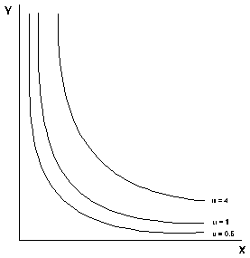
Figure 2 illustrates how it is possible to use a utility function to generate a diagram with the associated indifference curves. This figure illustrates Cobb-Douglas well-behaved preferences which are commonly employed in applied work.
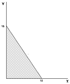
Up to this point, we have we have focused exclusively on the characterization of preferences. Let us now consider the other side of the consumer model – the budget constraint. The simplest approach to characterizing consumer income is to assume that the consumer has a fixed money income which she may spend on any goods. The only constraint on this choice is that the value of the expenditure may not exceed the money income. This is the standard budget constraint:
Graphically, this equation defines the line depicted in Figure 3. All points inside the budget line are affordable. The consumer faces a choice of which affordable bundle to select.
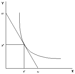
Within the framework of our theory, the answer is straightforward – the consumer will choose the one combination of x and y from the set of affordable bundles which maximizes her utility. This combination of x and y will be at the point where the indifference curve is tangent the budget line. This point is called the optimal choice. We see this illustrated in Figure 4.
The standard model of consumer behavior provides a starting point for learning MPSGE. This introduction is "hands on" – I will discuss issues as they arise, assuming that you have access to a computer and can invoke the program and read the output file. You may wish to learn the rudiments of GAMS syntax before starting out, although you may be able to pick up these ideas as they come, depending on your aptitude for computer languages.
Getting Started
For running MPSGE models, the GAMS/BASE module is required along with a suitable MCP solver such as MILES or PATH. To verify that the system is operational, run one of the MPSGE library models, e.g. SCARFMGE. This can be done easily via GAMS Studio (search for SCARFMGE in the Model Library Explorer). Alternatively, from a command prompt, connect to a working directory (never run models from the GAMS system directory!). Then, extract and run the model:
C:\>MKDIR WORK

C:\>CD WORK

C:\WORK>GAMSLIB SCARFMGE

C:\WORK>GAMS SCARFMGE
If the GAMS system is properly installed, these commands will cause GAMS to solve a sequence of models from the SCARFMGE sample problem. The output from this process is written to file SCARFMGE.LST . If you search for the word "STATUS", you can verify that all the cases are processed.
There are a number of MPSGE models included in the GAMS Model Library. If you are using a GAMS demo license, you will be able to process most but not all of the library models. The demo license limits the number of variables in the model to 1000.
Assuming that you have successfully installed the software, let us now proceed to some examples which illustrate both the computing syntax and the underlying economics.
Modeling Consumer Demand
Example 1: Evaluating a Demand Function
Consider a standard consumer choice problem, one which might appear on a midterm examination in intermediate microeconomics:
where 1 is the exogenous price of x and 2 is the price of y.
This type of problem is solved easily using GAMS/MINOS (as a nonlinear program). Strictly speaking, it is not the sort of model for which you would need to use MPSGE. At the same time, this can be an instructive example.
The key issue in this example is learning how to represent utility functions. MPSGE is "non-algebraic" – so function specification depends on an intuitive understanding of the underlying economic structure.
Consider Figure 5 and focus on a single point,
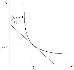
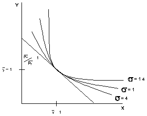
A utility function is represented in MPSGE by the specification of: (i) benchmark demand quantities, (ii) benchmark demand prices (iii) an elasticity of substitution at the benchmark point. Benchmark quantities determine an anchor point for the set of indifference curves. Benchmark prices fix the slope of the indifference curve at that point, and the elasticity describes the curvature of the indifference curve. Speaking formally, elasticities provide a "second order approximation" of the utility function. To understand the importance of the benchmark elasticity of substitution, consider Figure 6. This figure shows three indifference curves all of which share the same benchmark quantities and benchmark prices. They differ only in the elasticities of substitution. The least convex (flattest) curve has the highest elasticity, the most convex curve has the lowest elasticity. (When the elasticity of substitution is 0, the indifference curve is L-shaped with the corner at the benchmark point.)
Let us now consider how the consumer optimization problem can be cast as a general equilibrium model. We do this by adding a single factor of production and two "production" sectors. For concreteness, let the factor of production be called labor with a price PL. One production function converts one unit of labor into one unit of x, the other sector converts 2 units of labor into one unit ofy. Setting the labor endowment equal 120, the market clearance condition for labor reads:
which is precisely the budget constraint for the consumer's problem.
We will now present the program code, a few lines at a time. As part of working through the example, the student should type these lines into a file.
A MPSGE model specification is always listed between $ONTEXT and $OFFTEXT statements. The first statement within an MPSGE model-description assigns a name to the model. The model name must begin with a letter and must have 10 or fewer characters.
$ONTEXT

$MODEL:DEMAND
The model specification begins by declaring variables for the model. In a standard model, there are three types of variables: commodity prices, sectoral activity levels, and consumer incomes. The end of each line may include "! variable description ".
N.B. The variables associated with commodities are prices, not quantities. (In this and subsequent models, I use P as the first letter for each of the commodity variables to remind us that these variables are prices.)
N.B. The variable associated with a consumer is an income level, not a welfare index.
$SECTORS:
        X       ! ACTIVITY LEVEL FOR X = DEMAND FOR GOOD X
        Y       ! ACTIVITY LEVEL FOR Y = DEMAND FOR GOOD Y

$COMMODITIES:
        PX      ! PRICE OF X WHICH WILL EQUAL PL
        PY      ! PRICE OF Y WHICH WILL EQUAL 2 PL
        PL      ! PRICE OF THE ARTIFICIAL FACTOR L

$CONSUMERS:
        RA      ! REPRESENTATIVE AGENT INCOME
Function specifications follow the variable declarations. In this model, our first declarations correspond to the two production sectors. In this model, the production structures are particularly simple. Each of the sectors has one input and one output. In the MPSGE syntax, I: denotes an input and O: denotes an output. The output quantity coefficients for both sectors are unity (Q:1). This means that the level values for x and y correspond to the actual quantities produced. The final function specified in the model represents the utility function and endowments for our single consumer. In this function, the E: entries correspond to endowments and the D: entries are demands. Reference demands, reference prices and the substitution elasticity (s:1) characterize preferences.
The demand entries shown here are consistent with a Cobb-Douglas utility function in which the budget share for y is twice the budget share for x (i.e. the MRS at (1,1) equals 1/2):
$PROD:X
      O:PX  Q:1
      I:PL  Q:1

$PROD:Y
      O:PY  Q:1
      I:PL  Q:2

$DEMAND:RA  s:1
      E:PL  Q:120
      D:PX  Q:1   P:(1/2)
      D:PY  Q:1   P:1

$OFFTEXT
The final three statements in this file invoke the MPSGE preprocessor, "generate" and solve the model:
$SYSINCLUDE mpsgeset DEMAND

$INCLUDE DEMAND.GEN
SOLVE DEMAND USING MCP;
The preprocessor invocation ($SYSINCLUDE mpsgeset) should be placed immediately following the $OFFTEXT block containing the model description. The model generator code, DEMAND.GEN, is produced by the previous statement and must be referenced immediately before each subsequent SOLVE statement.
At this point, the reader should take the time to type the example into a file and execute the program with GAMS/MPSGE.
This is possibly the first GAMS model which some readers have solved, so it is worth looking through the listing file in some detail. After running the solver, we examine the listing file. I typically begin my assessment of a model's solution by searching for "STATUS". For this model, we have the following:
               S O L V E      S U M M A R Y

     MODEL   DEMAND
     TYPE    MCP
     SOLVER  PATH                FROM LINE  263

**** SOLVER STATUS     1 NORMAL COMPLETION
**** MODEL STATUS      1 OPTIMAL

 RESOURCE USAGE, LIMIT          1.432     1000.000
 ITERATION COUNT, LIMIT         5         1000
 EVALUATION ERRORS              0            0

 Work space allocated           --    4.86 Mb

Default price normalization using income for RA
This information is largely self-explanatory. The most important items are the SOLVER STATUS and MODEL STATUS indicators. When the solver status is 1 and the model status is 1, the system has returned an equilibrium.
For small models such as this, the limits on resource usage (time) and solver iterations have no effect. (You can modify these values with the statements:
 model.RESLIM  =  number of cpu seconds ;

 model.ITERLIM =  number of iterations ;
entered into the program before the SOLVE statement.)
The work space allocation for MPSGE models is determined by the number of variables in the model. It is possible to exogenously specify the work space allocation by assigning
model.WORKSPACE = xx ;
where xx is the desired number of megabytes.
The final message, "Default price normalization...", is significant. It reminds the user that an Arrow-Debreu general equilibrium model determines only relative prices. In such an equilibrium, the absolute scaling of prices is indeterminant. (I.e., if (p*,M*) are a set of equilibrium prices and income levels, then (2 p*,2 M*) is also a solution, etc.)
It is common practice in economics to address the normalization issue through the specification of a numeraire commodity. You can do this for an MPSGE model by "fixing" a price, with a statement like:
PX.FX = 1;
entered following the model declaration ($SYSINCLUDE mpsgeset) but prior to the solver invocation. When any price or income level is fixed, MPSGE recognizes that a numeraire has been specified and does no automatic normalization.
Following some output from the solver (PATH in this case), the listing file provides a complete report of equilibrium values. With MPSGE models, the equation listings are superfluous. The variable listings provide all the relevant information.
For this model, the solution listing appears as follows:
                       LOWER     LEVEL     UPPER    MARGINAL
---- VAR X               .       40.000     +INF       .
---- VAR Y               .       40.000     +INF       .
---- VAR PX              .        1.000     +INF       .
---- VAR PY              .        2.000     +INF       .
---- VAR PL              .        1.000     +INF       .
---- VAR RA              .      120.000     +INF       .

  X           SUPPLY AND DEMAND OF GOOD X
  Y           SUPPLY AND DEMAND OF GOOD Y
  PX          PRICE OF X WHICH WILL EQUAL CX * PL
  PY          PRICE OF Y WHICH WILL EQUAL CY * PL
  PL          PRICE OF THE ARTIFICIAL FACTOR L
  RA          REPRESENTATIVE AGENT INCOME
The LOWER and UPPER columns report variable bounds applied in the model. In these columns, zero is represented by "." and infinity is represented by "+INF". The LEVEL column reports the solution value returned by the algorithm. Here we see that the equilibrium price of x is 1 and the price of y is 2, as determined by the specification of labor inputs.
Exercises 1
(a) The utility function calibration point is arbitrary. Here, we have selected
(b) Increase the price of Q: coefficient for PL in sector Q: field for sector
(c) Compute an equilibrium in which commodity
Example 2: Evaluating the MRS
This example further explores the representation of demand functions with MPSGE. It sets up a trivial equilibrium model with two goods and one consumer which returns the marginal rate of substitution of good
When
In an equilibrium, final demand always equals endowments for both goods, because these are the only sources of demand and supply. The model as parameterized demonstrates that if we set endowments for this model equal to the demand function calibration point, the model equilibrium price ratio equals the benchmark MRS.
This program begins with some GAMS statements in which three scalar parameters are declared. These parameters will be used in the place of numbers within the MPSGE model. The syntax for these GAMS statements is introduced in Chapter 2 of the GAMS manual. In short, we declare
SCALAR
      X     QUANTITY OF X FOR WHICH THE MRS IS TO BE EVALUATED /1/
      Y     QUANTITY OF Y FOR WHICH THE MRS IS TO BE EVALUATED /1/
      MRS   COMPUTED MARGINAL RATE OF SUBSTITUTION;
The remainder of the <em>MPSGE</em> program is, in fact, simpler than Example 1.

$ONTEXT

$MODEL:MRSCAL

$COMMODITIES:
      PX    ! PRICE INDEX FOR GOOD X
      PY    ! PRICE INDEX FOR GOOD Y

$CONSUMERS:
      RA    ! REPRESENTATIVE AGENT

$DEMAND:RA  s:1
      D:PX  Q:1   P:(1/4)
      D:PY  Q:1   P:1
      E:PX  Q:X
      E:PY  Q:Y
$OFFTEXT
$SYSINCLUDE mpsgeset MRSCAL

$INCLUDE MRSCAL.GEN
SOLVE MRSCAL USING MCP;
Following the solution, we compute a function of the solution values, the ratio of the price of PX and PY and storing this result in the scalar MRS. This scalar value is then displayed in the listing file with 8 digits:
MRS = PX.L / PY.L;
OPTION MRS:8;
DISPLAY MRS;
Exercises 2
(a) Show that the demand function is homothetic by uniform scaling of the
(b)Modify the demand function calibration point so that the reference prices of both
Example 3: Leisure Demand and Labor Supply
This model investigates the labor-leisure decision. A single consumer is endowed with labor which is either supplied to the market or "repurchased" as leisure. The consumer utility function over market goods (
Goods
where goods LPROD is an index of labor productivity. An increase in productivity is equivalent to a proportional decrease in the prices of
The model declaration is as follows:
SCALAR          LPROD   AGGREGATE LABOR PRODUCTIVITY /1/,
                CX      COST OF X AT BASE YEAR PRODUCTIVITY /1/,
                CY      COST OF Y AT BASE YEAR PRODUCTIVITY /1/;
$ONTEXT

$MODEL:LSUPPLY

$SECTORS:
        X       ! SUPPLY=DEMAND FOR X
        Y       ! SUPPLY=DEMAND FOR Y
        LS      ! LABOR SUPPLY

$COMMODITIES:
        PX      ! MARKET PRICE OF GOOD X
        PY      ! MARKET PRICE OF GOOD Y
        PL      ! MARKET WAGE
        PLS     ! CONSUMER VALUE OF LEISURE

$CONSUMERS:
        RA      ! REPRESENTATIVE AGENT

$PROD:LS
        O:PL    Q:LPROD
        I:PLS   Q:1

$PROD:X
        O:PX    Q:1
        I:PL    Q:CX

$PROD:Y
        O:PY    Q:1
        I:PL    Q:CY

$DEMAND:RA  s:1
        E:PLS   Q:120
        D:PLS   Q:1     P:1
        D:PX    Q:1     P:1
        D:PY    Q:1     P:1

$OFFTEXT
$SYSINCLUDE mpsgeset LSUPPLY

$INCLUDE LSUPPLY.GEN
SOLVE LSUPPLY USING MCP;
We can use this model to evaluate the wage elasticity of labor supply. In the initial equilibrium (computed in the last statement) the demands for LPROD (below) increases labor productivity. After computing a new equilibrium, we can use the change in labor supply to determine the wage elasticity of labor supply, an important parameter in labor market studies. It should be emphasized that the elasticity of labor supply should be an input rather than an output of a general equilibrium model – this is a parameter for which econometric estimates can be obtained.
Here is how the programming works. First, we declare some scalar parameters which we will use for reporting, then save the "benchmark" labor supply in LS0:
SCALAR
      LS0   REFERENCE LEVEL OF LABOR SUPPLY
      ELS   ELASTICITY OF LABOR SUPPLY WRT REAL WAGE;

LS0 = LS.L;
Next, we modify the value of scalar LPROD, increasing labor productivity by 1%. Because this is a neoclassical model, this change is equivalent to increasing the real wage by 1%. We need to recompute equilibrium prices after having changed the LPROD value:
LPROD = 1.01;
$INCLUDE LSUPPLY.GEN
SOLVE LSUPPLY USING MCP;
We use this solution to compute and report the elasticity of labor supply as the percentage change in the LS activity:
ELS = 100 * (LS.L - LS0) / LS0;
DISPLAY ELS;
As the model is currently constructed, the wage elasticity of labor supply equals zero. This is because the utility function is Cobb-Douglas over goods and leisure, and the consumer's only source of income is labor. As the real wage rises, this increases both the demand for goods (labor supply) and the demand for leisure. These effect exactly balance out and the supply of labor is unchanged.
Exercises 3
(a) One way in which the labor supply elasticity might differ from zero in a model with Cobb-Douglas final demand is if there were income from some other source. Let the consumer be endowed with good
(b) A second way to "calibrate" the labor supply elasticity is to change the utility function. We can do this by changing the s:1 to s:SIGMA, where SIGMA is a scalar value representing the benchmark elasticity of substitution between SIGMA consistent with a labor supply elasticity equal to 0.15.
The Pure Exchange Model
Partial equilibrium analysis forms the basis of most economics courses at the undergraduate level. In these models we focus on price, supply and demand for a single commodity. The partial equilibrium approach neglects indirect effects, through which changes in the market for one good may influence the market for another good.
In the previous section, we focused on the choices of a single consumer. In the present section, we will explore the implications of interactions between many consumers with heterogeneous preferences. Furthermore, the analysis will explore the potentially important interaction between market prices and income which are determined jointly in a general equilibrium.
The most widely-used graphical framework for multi-agent exchange equilibrium analysis is the Edgeworth-Bowley box as illustrated in Figure 7. In this diagram we model the following economy:
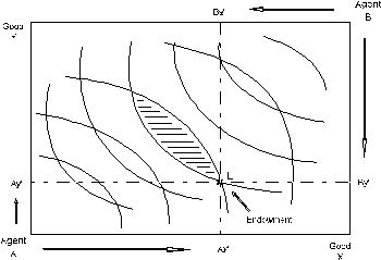
- Two types of consumers, denoted
and . We consider and to each represent multiple consumers, each with the same endowments and preferences. This assumption is helpful for justifying our assumption of perfectly competitive, price-taking behavior. - Two commodities, denoted
and - Fixed endowments of both goods. The horizontal axis measures the total world endowment of good
. The vertical axis measure the total world endowment of good . Any point in the box then represents an allocation of goods between the two agents. The agent allocation is measured with respect to the lower left origin. The agent allocation is measured with respect to the upper right origin.
Each agent has a given initial endowment, here denoted point
The key idea in this model is that trade can improve both agents' welfare. One agent gives some amount good
- Trade is mutually beneficial. So long as the transactions are voluntary, neither
nor will be hurt by engaging in trade. - Market prices can be used to guide the economy to a Pareto-efficient allocation, a state of affairs in which further mutually-beneficial trades are not possible.
- There is no guarantee that the gains from trade will be "fairly distributed" across consumers. A competitive equilibrium may produce a significant welfare increase for one consumer while have negligible impact on the other.
- There are multiple Pareto-efficient allocations, typically only one of which is a competitive equilibrium. We can use this model to demonstrate that the issues of efficiency and equity can be separated when there is the possibility of lump-sum income transfers between agents.
Modeling Pure Exchange with MPSGE
Example 4: A 2x2 Exchange Model
In this program, we examine the simple two good, two agent model of exchange equilibrium. The world endowments for goods
SCALAR  XA              AGENT A ENDOWMENT OF X ( 0 < XA < 1)    /0.2/
        YA              AGENT A ENDOWMENT OF Y ( 0 < YA < 1)    /0.8/
        THETA_A         AGENT A DEMAND SHARE PARAMETER FOR X    /0.5/
        THETA_B         AGENT B DEMAND SHARE PARAMETER FOR X    /0.8/
        SIGMA_A         AGENT A ELASTICITY PARAMETER            /2.0/
        SIGMA_B         AGENT B ELASTICITY PARAMETER            /0.5/;
This model is actually simpler than the models presented above because we have no need for production. There are simply two commodities and two consumers. The consumers differ in terms of commodity endowments and preferences. The competitive equilibrium prices are such that supply equals demand for both goods and both agents spend an amount equal to their endowment income.
This model illustrates how to use computed function coefficients. See, for example, Q:(1-THETA_A) in the $DEMAND:A block. Any numeric input field in an MPSGE model may be "computed", provided that the algebraic expression is enclosed within parentheses and legitimate GAMS code.
This model specification uses the default values for reference prices in the demand function blocks. When P:value is not specified in a D:,I: or O: record, P:1 is assumed.
This model uses the more general constant-elasticity-of-substitution utility function.
$ONTEXT

$MODEL:EXCHANGE

$COMMODITIES:
      PX    ! EXCHANGE PRICE OF GOOD X
      PY    ! EXCHANGE PRICE OF GOOD Y

$CONSUMERS:
      A     ! CONSUMER A
      B     ! CONSUMER B

$DEMAND:A  s:SIGMA_A
      E:PX  Q:XA
      E:PY  Q:YA
      D:PX  Q:THETA_A
      D:PY  Q:(1-THETA_A)

$DEMAND:B  s:SIGMA_B
      E:PX  Q:(1-XA)
      E:PY  Q:(1-YA)
      D:PX  Q:THETA_B
      D:PY  Q:(1-THETA_B)

$OFFTEXT
$SYSINCLUDE mpsgeset EXCHANGE

$INCLUDE EXCHANGE.GEN
SOLVE EXCHANGE USING MCP;

SCALAR
      PRATIO  EQUILIBRIUM PRICE OF X IN TERMS OF Y,
      IRATIO  EQUILIBRIUM RATIO OF CONSUMER A INCOME TO CONSUMER B INCOME;

PRATIO = PX.L / PY.L;
IRATIO = A.L  / B.L;

DISPLAY IRATIO, PRATIO;
The foregoing sets up the model and computes the competitive equilibrium. After GAMS returns from the solver, we declare and compute some report values.
Absolute levels of income and price returned from a general equilibrium model are not meaningful because a model determines only relative prices. For this reason, we report equilibrium income and price levels in relative terms.
In the final step, we compute an alternative efficient equilibrium, one in which the income levels for A and B are equal. The purpose of this exercise is to demonstrate the second welfare theorem. When incomes are both fixed, the equilibrium remains efficient, but the connection between market prices and endowment income is eliminated.
In GAMS/MPSGE, a variable may be fixed using the GAMS syntax
variable.fx= value;
as illustrated in this model:
A.FX = 1;
B.FX = 1;
$INCLUDE EXCHANGE.GEN
SOLVE EXCHANGE USING MCP;

SCALAR      TRANSFER  IMPLIED TRANSFER FROM A TO B AS A PERCENTAGE OF INCOME;

TRANSFER = 100 * ( A.L - PX.L * XA - PY.L * YA ); PRATIO = PX.L / PY.L;
IRATIO = A.L  / B.L;

DISPLAY TRANSFER, PRATIO, IRATIO;
Exercises 4
(a) Set up a separate models which computes the autarchy price ratios for consumers A and B. (You can use one of the earlier models as a starting point.)
(b) Determine parameter values for which the endowment point is the equilibrium point.
(c) Set up a series of computations from which you can sketch the efficiency locus. Draw the Edgeworth box diagram which is consistent with these values.
Example 5: Import Tariffs and Market Power
The exchange model provides a remarkably useful tool for analyzing issues related to international trade. Formal trade theory is more complicated with the inclusion of separate production technologies. We will present some of those models below. Before going forward, however, we will consider a slight generalization of the 2x2 model exchange model. In this extension, we introduce independent markets for consumers A and B and trade activities which deliver goods from one market to the other.
The set of input parameters largely the same as in the previous example. Two new parameters are ad-valorem tariffs which apply on imports to each of the regions.
SCALAR  XA              AGENT A ENDOWMENT OF X ( 0 le XA le 1)    /0.2/
        YA              AGENT A ENDOWMENT OF Y ( 0 le YA le 1)    /0.8/
        THETA_A         AGENT A DEMAND SHARE PARAMETER FOR X    /0.4/
        THETA_B         AGENT B DEMAND SHARE PARAMETER FOR X    /0.6/
        SIGMA_A         AGENT A ELASTICITY PARAMETER            /1.0/
        SIGMA_B         AGENT B ELASTICITY PARAMETER            /1.0/,
        T_A             AD-VALOREM TARIFF ON IMPORTS TO AGENT A /0.10/
        T_B             AD-VALOREM TARIFF ON IMPORTS TO AGENT B /0.10/;
The program differs from the previous example in several respects. First, we introduce a separate commodity price for each agent. In the absence of tariffs, these prices are identical.
A second difference is that in this model trade activities deliver goods from one agent to the other. These are denoted M{good}{agent} for imports of {good} to {agent}. There are four flows which may be operated in only one direction (the activity levels are non-negative). In terms of initial endowments and preferences, this model has exactly the same economic structure as the previous model.
$ONTEXT

$MODEL:TARIFFS

$SECTORS:
        MXA     ! TRADE IN X FROM B TO A
        MXB     ! TRADE IN X FROM A TO B
        MYA     ! TRADE IN Y FROM B TO A
        MYB     ! TRADE IN Y FROM A TO B


$COMMODITIES:
        PXA     ! PRICE OF GOOD X FOR AGENT A
        PYA     ! PRICE OF GOOD Y FOR AGENT A
        PXB     ! PRICE OF GOOD X FOR AGENT B
        PYB     ! PRICE OF GOOD Y FOR AGENT B

$CONSUMERS:
        A       ! CONSUMER A
        B       ! CONSUMER B

$DEMAND:A  s:SIGMA_A
        E:PXA   Q:XA
        E:PYA   Q:YA
        D:PXA   Q:THETA_A
        D:PYA   Q:(1-THETA_A)

$DEMAND:B  s:SIGMA_B
        E:PXB   Q:(1-XA)
        E:PYB   Q:(1-YA)
        D:PXB   Q:THETA_B
        D:PYB   Q:(1-THETA_B)
The trade activities each have one input and one output. They simply deliver a good ( "A:" which specifies the tax agent, a consumer who collects the tax revenue as part of income. The second is "T:" which specifies the ad- valorem tax rate.
MPSGE permits taxes to applied on production inputs and outputs but it does not permit taxes on final demand.
The tax applies on a net basis on inputs. For example, if we consider the MXA sector, the price of one unit of input is given by:
where
$PROD:MXA
      O:PXA Q:1
      I:PXB Q:1   A:A  T:T_A

$PROD:MXB
      O:PXB Q:1
      I:PXA Q:1   A:B  T:T_B

$PROD:MYA
      O:PYA Q:1
      I:PYB Q:1   A:A  T:T_A

$PROD:MYB
      O:PYB Q:1
      I:PYA Q:1   A:B  T:T_B
The final portions of the file introduces one use of "MPSGE report variables". In this case, report variables are used to recover a Hicksian money-metric welfare index for each of the agents. We compute the initial, tariff-ridden equilibrium in order to compute the benchmark welfare levels. We then set all tariffs to zero and compute the free-trade equilibrium. Using the final welfare indices and the saved values of the benchmark welfare levels, we are able to report the change in welfare from removing tariff distortions.
$REPORT:
      V:WA  W:A
      V:WB  W:B

$OFFTEXT
$SYSINCLUDE mpsgeset TARIFFS

$INCLUDE TARIFFS.GEN
SOLVE TARIFFS USING MCP;

SCALAR
      WA0   BENCHMARK WELFARE INDEX FOR AGENT A
      WB0   BENCHMARK WELFARE INDEX FOR AGENT B;

WA0 = WA.L;
WB0 = WB.L;
T_A = 0;
T_B = 0;

$INCLUDE TARIFFS.GEN
SOLVE TARIFFS USING MCP;

SCALAR
      EVA   HICKSIAN EQUIVALENT VARIATION FOR AGENT A
      EVB   HICKSIAN EQUIVALENT VARIATION FOR AGENT B;

EVA = 100 * (WA.L-WA0)/WA0;
EVB = 100 * (WB.L-WB0)/WB0;
DISPLAY EVA, EVB;
Exercises 5
(a) Find the "optimal tariff" in this model for agent A, assuming that agent B does not retaliate and leaves her tariff rate at the benchmark level.
(b) Insert the endowment and preference parameters from the previous problem, retaining the same "benchmark" tariff rates. Does free trade benefit both countries? If not, why not?