Table of Contents
- Date
- 16 April 2013
Introduction
ANTIGONE, Algorithms for coNTinuous / Integer Global Optimization of Nonlinear Equations, is a deterministic general mixed-integer nonlinear global optimization framework [133, 134, 135, 136, 137] .
where
where the powers
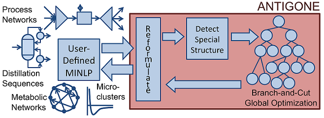
As illustrated in the following figure, ANTIGONE responds dynamically to exploit special structure within (MINLP). ANTIGONE falls broadly into the category of branch-and-bound global optimization because it: generates and solves convex relaxations of the nonconvex MINLP that rigorously bound the global solution; finds feasible solutions via local optimization; divides and conquers the feasible set to generate a sequence of convex relaxations converging to the global optimum [65, 64] .
Licensing and software requirements
Using GAMS/ANTIGONE requires
- an ANTIGONE license,
- a CPLEX license, and
- a CONOPT or SNOPT license.
Running GAMS/ANTIGONE
GAMS/ANTIGONE solves: NLP; MINLP; RMINLP; QCP; MIQCP; RMIQCP; CNS. If GAMS/ANTIGONE is not the default solver for these models, it can be called using the following command before the solve statement:
option nlp=antigone, minlp=antigone, rminlp=antigone;
GAMS/ANTIGONE Output
The log output shown below is generated using the MINLP model cecil_13 from the MINLPLib.
-------------------------------------------------------------------------------
ANTIGONE: Algorithms for coNTinuous/Integer Global Optimization; Version 1.0

          Ruth Misener and Christodoulos A. Floudas

          Computer-Aided Systems Laboratory (CASL)
          Department of Chemical & Biological Engineering; Princeton University
-------------------------------------------------------------------------------

Before Pre-processing:
          840 Variables
                 660 Continuous
                 180 Binary
          929 Equations

After Pre-processing:
          520 Variables
                 418 Continuous
                 102 Binary
          499 Equations
                 291 Linear
                 208 Nonconvex nonlinear
          232 Nonlinear Terms
                 232 Signomial
          730 Possible Reformulation Linearization Technique (RLT) equations
             34 RLT Equations Added Outright to Formulation

Constituent Libraries:
            CPLEX  Solving relaxations
            CONOPT Finding feasible points
            LAPACK Addressing linear systems
            Boost  Bounding Intervals

-------------------------------------------------------------------------------
Time (s) Nodes explored Nodes remaining Best possible   Best found Relative Gap
-------------------------------------------------------------------------------

      65              1               1    -1.158e+05   -1.157e+05   +1.032e-03
     134              1               1    -1.157e+05   -1.157e+05   +4.337e-04
     202              1               1    -1.157e+05   -1.157e+05   +4.334e-04
     258              1               1    -1.157e+05   -1.157e+05   +4.140e-06
     Solving MILP relaxation at tree level 0 ----------------------------------
     341              1               1    -1.157e+05   -1.157e+05   +4.091e-06
     413              1               1    -1.157e+05   -1.157e+05   +4.011e-06
     Solving MILP relaxation at tree level 0 ----------------------------------
     483              1               1    -1.157e+05   -1.157e+05   +4.001e-06
     571              1               1    -1.157e+05   -1.157e+05   +3.959e-06
     Solving MILP relaxation at tree level 0 ----------------------------------
     640              1               1    -1.157e+05   -1.157e+05   +3.880e-06
     Solving MILP relaxation at tree level 0 ----------------------------------
     702              1               0    -1.157e+05   -1.157e+05   +1.000e-06

-------------------------------------------------------------------------------
Termination Status : Global minimum
Best Feasible Point: -1.156565e+05
Best Possible Point: -1.156566e+05
       Relative Gap: +1.000000e-06
Algorithm analysis :

                  0 Nodes explored
                  0 Nodes remaining

                  0 Maximum tree depth

                183 Cutting Planes (183 Globally Valid)
                       183 Signomial

             702.38 Total time (CPU s)
                      0.07 Pre-processing
                    698.56 Solving MILP relaxations
                      0.95 Searching for feasible solutions
                      2.79 Variable bounds tightening
                             2.31 OBBT
                             1.48 FBBT (0.13 EC; 0.92 RLT; 0.00 Factoring)
                      0.00 Branching
                             0.00 Reliability branching
-------------------------------------------------------------------------------
Summary of ANTIGONE Options
General Options
| Option | Description | Default |
|---|---|---|
| abs_opt_tol | absolute stopping tolerance | GAMS optca |
| dumpsolutions | name of solutions index gdx file for writing alternate solutions | |
| max_number_nodes | node limit | GAMS nodlim |
| max_time | resource limit | GAMS reslim |
| readparams | read secondary option file in ANTIGONE syntax | |
| rel_opt_tol | relative stopping tolerance | GAMS optcr |
| trydual | call CONOPT or SNOPT to produce duals | 5 |
Options for Solving the MILP Relaxations
| Option | Description | Default |
|---|---|---|
| cplex_optfile | read a secondary GAMS/CPLEX options file that will be applied to every LP and MILP subsolve | |
| cut_generation_epsilon | absolute violation threshold for separating hyperplanes | 1e-4 |
| nominal_time_limit | nominal time limit for solving MILP subproblems | 100 |
| populate_solution_pool | emphasis on generating starting points | 3 |
Options for Finding Feasible Solutions
| Option | Description | Default |
|---|---|---|
| conopt_optfile | read a secondary GAMS/CONOPT options file that will be applied to every NLP subsolve | |
| feas_soln_time_limit | time limit (s) for an NLP solve | 30 |
| feas_tolerance | absolute feasibility tolerance | 1e-6 |
| nlp_solver | use CONOPT or SNOPT to find feasible solutions | conopt |
Options for Branching
| Option | Description | Default |
|---|---|---|
| branching_bounds_push_away | branch a minimum fraction away from the variable bounds | 0.1 |
| branching_weight | branch on a convex combination of midpoint and solution | 0.25 |
| num_reliability_tests | number of strong branching initialization tests | 8 |
| reliability_branching | heuristic choice for building reliable pseudocosts | error |
| reliability_branching_mu | score parameter for building reliability | 0.15 |
| use_reliability_branching | use reliability branching? | 1 |
Options for Bounding
| Option | Description | Default |
|---|---|---|
| fbbt_improvement_bound | bounds reduction improvement threshold needed to exit FBBT loop | 0.999 |
| max_fbbt_iterations | maximum number of FBBT iterations | 50 |
| max_obbt_iterations | maximum number of OBBT iterations | 30 |
| max_time_each_obbt | time limit (s) for each OBBT LP | 10 |
| obbt_improvement_bound | bounds reduction improvement threshold | 0.95 |
| use_obbt | use optimality-based bounds tightening? | 1 |
Options for Logging to the Console
| Option | Description | Default |
|---|---|---|
| logging_freq | how often should we log progress to the console? | 5 |
| logging_level | logging information level | -1 |
| print_options | print the option parameter choices used in a single run? | 1 |
Options for Addressing Special Structure
| Option | Description | Default |
|---|---|---|
| adaptive_add_rlt | use the dynamic approach to adaptively determine deep RLT cuts? | 1 |
| adaptive_add_rlt_tree_depth | tree depth for heuristic that adaptively determines deep RLT cuts | 3 |
| add_bilinear_terms | allow addition of nonconvex bilinear terms to generate deep RLT cuts | 1 |
| convexity_cuts | derive convexity-based separating cuts for multivariable terms? | 1 |
| dominant_ec_only | add only the low-dimension edge-concave aggregations introducing dominant cuts into relaxations? | 1 |
| eigenvector_projections | use eigenvector projections as additional cuts? | 1 |
| eigenvector_projection_partitioning | allow partitioning on eigenvector projections? | 1 |
| low_dim_edge_concave_agg | use low-dimension edge-concave aggregations? | 1 |
| max_partitioned_quantities | number of partitioned quantities | 0 |
| max_rlt_cuts | maximum number of violated RLT cuts to add before resolving the relaxation? | 100 |
| naive_add_ec | naively integrate all low-dimension edge-concave aggregations into relaxations? | 0 |
| naive_add_rlt | naively add all RLT cuts to the relaxations? | 0 |
| number_of_partitions | how many partitions per variable? | 1 |
| partitioning_scheme | Partitioning scheme can be linear or logarithmic | linear |
| piecewise_linear_partitions | use piecewise-linear partitioning? | 0 |
| rlt | find RLT variable/equation and equation/equation pairs? | 1 |
| use_alpha_bb | apply globally-valid alphaBB cuts to tighten a node relaxation | 1 |
| use_edge_concave_dynamic | apply locally-valid edge-concave cuts to tighten a node relaxation | 1 |
In addition, GAMS option threads specifies the number of processors to use for linear algebra routines, e.g., when computing eigenvalues of a quadratic coefficients matrix. By default, all available processors are used.
Detailed Descriptions of ANTIGONE Options
abs_opt_tol (real): absolute stopping tolerance ↵
Default:
GAMS optca
adaptive_add_rlt (boolean): use the dynamic approach to adaptively determine deep RLT cuts? ↵
In the first few levels of the branch-and-bound tree, query the RLT equations after solving an initial relaxation. Add violated equations to the relaxation and resolve. Track the most commonly-violated equations and include those cuts in later nodes.
Default:
1
adaptive_add_rlt_tree_depth (integer): tree depth for heuristic that adaptively determines deep RLT cuts ↵
To the specified tree depth, solve the relaxation of a node twice if RLT equations are violated. After this depth, automatically add the most commonly violated cuts to the solution of each node
Range: {
1, ...,100}Default:
3
add_bilinear_terms (boolean): allow addition of nonconvex bilinear terms to generate deep RLT cuts ↵
Default:
1
branching_bounds_push_away (real): branch a minimum fraction away from the variable bounds ↵
Range: [
0,0.5]Default:
0.1
branching_weight (real): branch on a convex combination of midpoint and solution ↵
The branching weight specifies the emphasis on the midpoint of a variable, so larger branching weights imply branching closer to the center of a variable range.
Range: [
0,1]Default:
0.25
conopt_optfile (string): read a secondary GAMS/CONOPT options file that will be applied to every NLP subsolve ↵
Gain direct access to the GAMS/CONOPT options. The value of the string should match the name of the GAMS/CONOPT options file.
convexity_cuts (boolean): derive convexity-based separating cuts for multivariable terms? ↵
Default:
1
cplex_optfile (string): read a secondary GAMS/CPLEX options file that will be applied to every LP and MILP subsolve ↵
Gain direct access to the GAMS/CPLEX options. Specifying an options file allows, for example, the possibility of running the CPLEX subsolver with multiple threads. The value of the string should match the name of the GAMS/CPLEX options file.
cut_generation_epsilon (real): absolute violation threshold for separating hyperplanes ↵
Absolute violation threshold to generate separating hyperplanes for convex multivariable terms
Range: [
1e-7,10]Default:
1e-4
dominant_ec_only (boolean): add only the low-dimension edge-concave aggregations introducing dominant cuts into relaxations? ↵
Default:
1
dumpsolutions (string): name of solutions index gdx file for writing alternate solutions ↵
The GDX file specified by this option will contain a set call
indexthat contains the names of GDX files with the individual solutions. For details see example model dumpsol in the GAMS Test Library.
eigenvector_projections (boolean): use eigenvector projections as additional cuts? ↵
Default:
1
eigenvector_projection_partitioning (boolean): allow partitioning on eigenvector projections? ↵
Default:
1
fbbt_improvement_bound (real): bounds reduction improvement threshold needed to exit FBBT loop ↵
Range: [
0,1]Default:
0.999
feas_soln_time_limit (real): time limit (s) for an NLP solve ↵
Range: [
1, ∞]Default:
30
feas_tolerance (real): absolute feasibility tolerance ↵
Default:
1e-6
logging_freq (real): how often should we log progress to the console? ↵
Wait at least the specified time in seconds before next output to the console
Range: [
1, ∞]Default:
5
logging_level (integer): logging information level ↵
Log to the console at the specified level (-1: default; 0: minimal logging; 3: extensive logging)
Default:
-1
value meaning -1minimal plus warnings 0minimal 1entering info 2updating info 3includes Cplex updates
low_dim_edge_concave_agg (boolean): use low-dimension edge-concave aggregations? ↵
Default:
1
max_fbbt_iterations (integer): maximum number of FBBT iterations ↵
Range: {
1, ...,100}Default:
50
max_number_nodes (integer): node limit ↵
Default:
GAMS nodlim
max_obbt_iterations (integer): maximum number of OBBT iterations ↵
Range: {
1, ...,100}Default:
30
max_partitioned_quantities (integer): number of partitioned quantities ↵
Range: {
0, ...,50}Default:
0
max_rlt_cuts (integer): maximum number of violated RLT cuts to add before resolving the relaxation? ↵
Range: {
1, ...,1000}Default:
100
max_time (real): resource limit ↵
Default:
GAMS reslim
max_time_each_obbt (real): time limit (s) for each OBBT LP ↵
Range: [
1,100]Default:
10
naive_add_ec (boolean): naively integrate all low-dimension edge-concave aggregations into relaxations? ↵
Default:
0
naive_add_rlt (boolean): naively add all RLT cuts to the relaxations? ↵
Default:
0
nlp_solver (string): use CONOPT or SNOPT to find feasible solutions ↵
Note, that independent of the setting for this option, for the initial NLP solve from the user provided starting point, always CONOPT is used, if available. Further, for the final NLP solve (see trydual), always CONOPT is used, if available, otherwise SNOPT is used.
Default:
conopt
value meaning conoptConopt snoptSnopt
nominal_time_limit (real): nominal time limit for solving MILP subproblems ↵
Nominal time limit for solving MILP subproblems. Terminate long-running MILP subproblems over this time limit once they reach an integer feasible point
Range: [
0.1,1000]Default:
100
number_of_partitions (integer): how many partitions per variable? ↵
Range: {
0, ...,16}Default:
1
num_reliability_tests (integer): number of strong branching initialization tests ↵
Range: {
1, ...,100}Default:
8
obbt_improvement_bound (real): bounds reduction improvement threshold ↵
Bounds reduction improvement threshold needed to exit OBBT loop This parameter also determines whether to continue obbt in child; if the parent bound improvement is less than this threshold, then child node won't try OBBT
Range: [
0,1]Default:
0.95
partitioning_scheme (string): Partitioning scheme can be linear or logarithmic ↵
Linear partitioning uses a number of binary variables linear in the number of partitions while logarithmic partitioning uses a number of binary variables logarithmic in the number of breakpoints. Linear partitioning tends to be numerically favorable for a few breakpoints while logarithmic partitioning is better for a larger number of breakpoints.
Default:
linear
value meaning linearLinear partitioning logarithmicLogarithmic partitioning
piecewise_linear_partitions (boolean): use piecewise-linear partitioning? ↵
Default:
0
populate_solution_pool (integer): emphasis on generating starting points ↵
Emphasis on generating many starting points for NLP solves using the CPLEX solution pool feature. Larger number implies more starting points.
Range: {
0, ...,4}Default:
3
print_options (boolean): print the option parameter choices used in a single run? ↵
Default:
1
readparams (string): read secondary option file in ANTIGONE syntax ↵
reliability_branching (string): heuristic choice for building reliable pseudocosts ↵
Default:
error
value meaning errorMax Error Branching forwardForward branching reverseReverse branching
reliability_branching_mu (real): score parameter for building reliability ↵
Range: [
0,1]Default:
0.15
rel_opt_tol (real): relative stopping tolerance ↵
Default:
GAMS optcr
rlt (boolean): find RLT variable/equation and equation/equation pairs? ↵
Default:
1
trydual (real): call CONOPT or SNOPT to produce duals ↵
Spend the specified amount of time in seconds or less in producing a dual solution by calling CONOPT or SNOPT.
Range: [
0, ∞]Default:
5
use_alpha_bb (boolean): apply globally-valid alphaBB cuts to tighten a node relaxation ↵
Default:
1
use_edge_concave_dynamic (boolean): apply locally-valid edge-concave cuts to tighten a node relaxation ↵
Default:
1
use_obbt (boolean): use optimality-based bounds tightening? ↵
Default:
1
use_reliability_branching (boolean): use reliability branching? ↵
Default:
1
ANTIGONE Algorithmic Features
As illustrated in the figure above, the primary algorithmic features in ANTIGONE are reformulating model input, elucidating special structure, and branch-and-bound global optimization [133, 134, 135, 136, 137] .
Reformulating Model Input
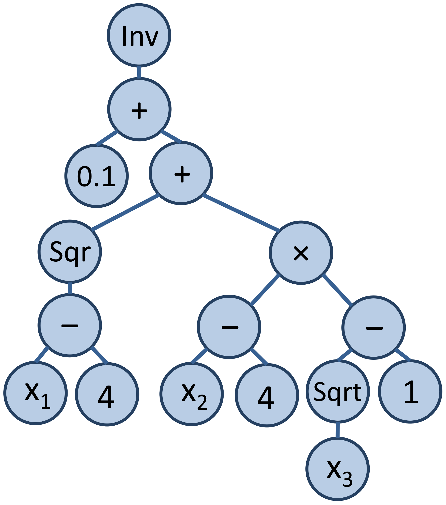
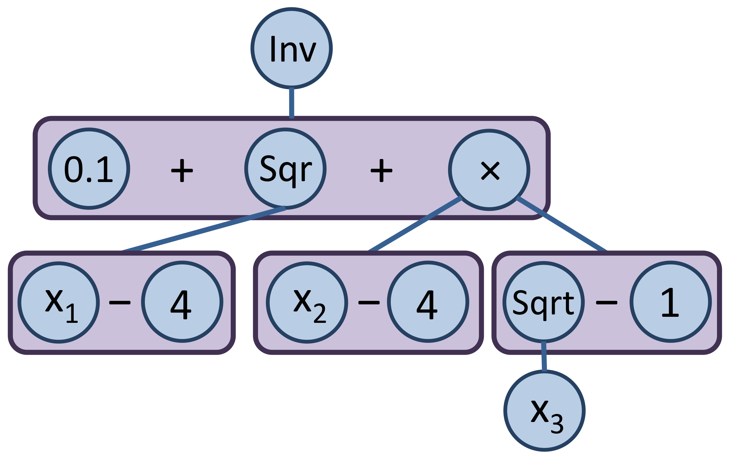
As illustrated in the figure below, ANTIGONE transforms a factorable programming tree into a flattened expression tree to capitalize on the development of tight convex underestimators for specific classes of nonlinear terms. ANTIGONE extends the efficacy of hybrid strategies by meaningfully integrating mutually reinforcing operator- and term-based strategies [26, 75, 136] . This approach reformulates towards multivariable terms with specialized underestimators while maintaining a tree-like representation of powers that cannot be distributed and convex operators that can be exploited by dynamic cut generation.
 |
 |
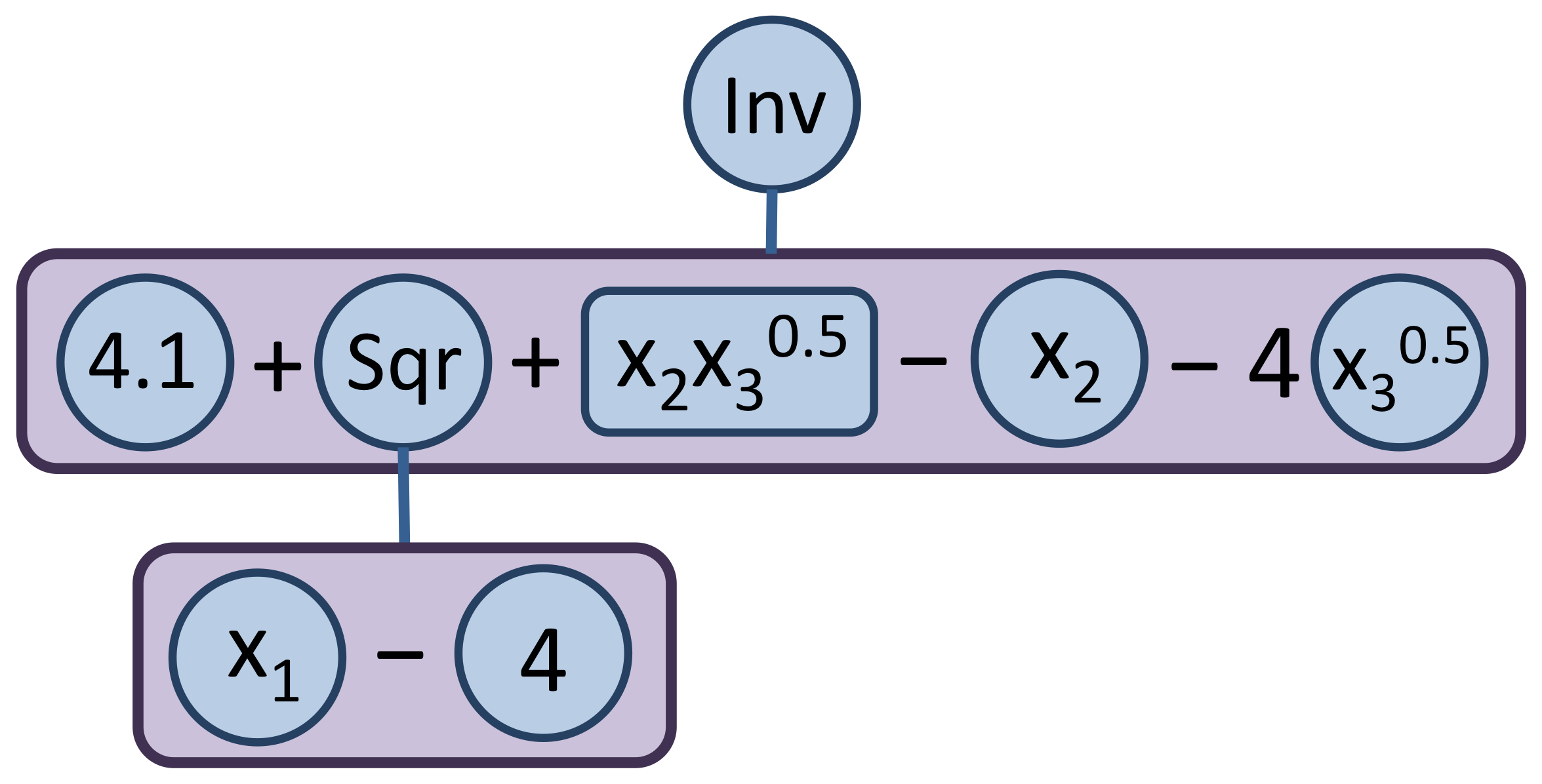 |
| (a) Binary Expression Tree | (b) Factorable Programming Tree | (c) Flattened Expression Tree |
Elucidating Special Structure
After reformulating the user-defined MINLP, ANTIGONE detects special mathematical structure that it will exploit in the branch-and-cut phase (Section Branch-and-Bound Global Optimization). The types of special structure that ANTIGONE considers are: reformulation-linearization technique (RLT) equations; convexity/concavity; edge-convexity/edge-concavity;
- RLT multiplies every pairwise combination of: variables; nonlinear terms; equations [10, 118, 134, 136, 137, 172, 168, 169, 170, 171] . ANTIGONE saves the combinations that do not introduce new terms into the model formulation and updates these equations at every node of the branch-and-cut tree. Special RLT equations are added directly to the model formulation; other RLT equations are used as cutting planes and integrated into the feasibility-based bounds tightening routines.
- Convexity/Concavity permits the easy generation of a cutting plane at a point
Based on interval arithmetic, terms and multi-term expressions are labeled as always/sometimes/never convex/ concave; this information is used in the branch-and-cut phase. - Edge-Convexity/Edge-Concavity implies a vertex polyhedral envelope; ANTIGONE labels terms and multi-term expressions as always/sometimes/never edge-convex/edge-concave with a simple interval arithmetic test [132, 176, 174, 175] .
- Term-Specific Underestimators are diagrammed in the figure below; their implementation is based on work available in the open literature [51, 52, 66, 76, 117, 124, 122, 123, 128, 132, 133, 145, 176, 174, 177] .
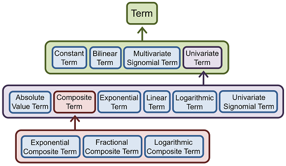 Inheritance Structure of Base Class Term
Branch-and-Bound Global Optimization
After the reformulation and special structure detection phases, ANTIGONE initiates a branch-and-cut global optimization algorithm that generates tight convex underestimators, dynamically generates separating hyperplanes, bounds the variables [5, 9, 4, 10, 17, 48, 49, 115, 156, 157, 170, 171, 190]; branches on the search space [1, 17], and finds feasible solutions.