Table of Contents
Introduction
In multi-objective optimization (MOO) there is more than one objective function and there is no single optimal solution that simultaneously optimizes all the objective functions. In MOO the concept of optimality is replaced by Pareto efficiency or optimality. Pareto efficient (or optimal, nondominated, etc.) solutions are solutions that cannot be improved in one objective without deteriorating in at least one of the other objectives. The mathematical definition of an efficient solution is the following:
Without loss of generality assume that all objective functions \(f_k\) with \(k=1,...,p\) are for minimization. A feasible solution \(x\) of a MOO problem is (strongly) efficient if there is no feasible solution \(x'\) such as \(f_k(x') \leq; f_k(x)\) for \(k=1,...,p\) with at least one strict inequality. A feasible solution \(x\) is weakly efficient if there is no feasible solution \(x'\) such as \(f_k(x') < f_k(x)\) for \(k=1,...,p\).
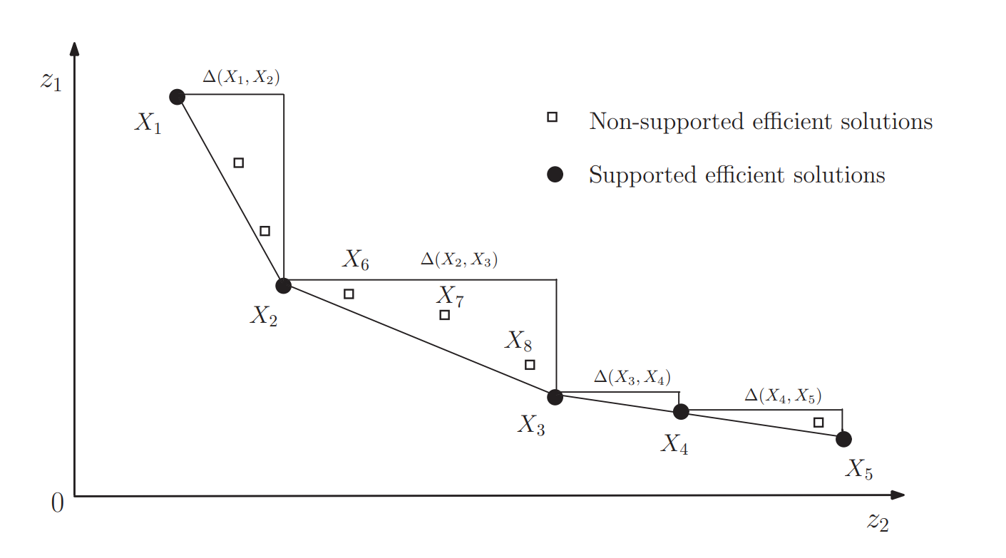
In case of a non-convex feasible objective and decision space (e.g. MIP), the set of efficient solutions can be further partitioned into supported and non-supported efficient solutions. Supported efficient solutions are optimal solutions of the weighted sum single objective problem for any non-negative weights (corner solutions of the feasible space). See the following graph that illustrates the difference between supported and non-supported efficient solutions:
A simple MOO method is lexicographic optimization. Lexicographic optimization presumes that the decision-maker has lexicographic preferences, ranking the efficient solutions to a lexicographic order of the objective functions. A lexicographic minimization problem can be written as:
\(lex\) \(min\) \(f_1(x),f_2(x),...,f_p(x)\)
s.t.
\(x \in S\)
where \(x\) is the vector of decision variables, \(S\) is the feasible region, and \(f_1(x),f_2(x),...,f_p(x)\) are the \(p\) objective functions ordered from the most to the least important. A lexicographic minimization problem with \(p\) objective functions can be solved using a sequence of \(p\) single-objective optimization problems as follows:
For \(i=1,...,p\) do
Solve single-objective optimization problem:
\(min\) \(z_i\)
s.t.
\(f_k(x)=z_k\) \(\forall k=1,...,i-1\)
\(x \in S\)where \(z_k\) are the objective function variables
- Fix the value of objective function variable \(z_i\) for the following iterations
End for
The Payoff method provided by this LibInclude file uses lexicographic optimization to calculate a payoff table. The \(p \times p\) payoff table contains the results of \(p\) lexicographic optimizations with orders \( \lbrace f_1(x),f_2(x),...,f_p(x) \rbrace , \lbrace f_2(x),f_3(x),...,f_p(x),f_1(x) \rbrace , ..., \lbrace f_p(x),f_1(x),...,f_{p-1}(x) \rbrace \). Other MOO methods provided by this LibInclude file use the Payoff method to obtain e.g. ranges for the objectives.
This LibInclude file provides a collection of methods to generate Pareto efficient solutions for MOO models. All implemented methods are so-called a-posteriori (or generation) methods for generating Pareto efficient solutions. After the Pareto efficient set or a representative subset of the Pareto efficient set has been generated, it is returned to the user, who then analyses the solutions and selects the most preferred among the alternatives.
Usage
LibInclude file moo.gms provides methods for multi-objective optimization in GAMS and can be used as follows:
$libinclude moo method modelName modelType objectiveSet direction objectiveVar points paretoPoints [optList]
Where:
Argument Description methodSpecify the name of the method to use. Available methods are EpsConstraint,Payoff,RandomWeighting, andSandwiching. See Methods for details.modelNameSpecify the name of the multi-objective optimization model that should be solved. modelTypeSpecify the corresponding model type, e.g. LP.objectiveSetSpecify the set of objectives. directionOne-dimensional parameter that contains the optimization direction for each objectiveSetelement - min (-1) or max (+1).objectiveVarSpecify the objective function variable. Compared to the traditional scalar objective function variable with a single objective optimization problem in GAMS, this objective function variable is one-dimensional. pointsSpecify the set of pareto points. The number of members in the set defines the maximum number of returned pareto points. Therefore, make sure to define the set large enough. paretoPointsSpecify the two-dimensional ( points,objectiveSet) parameter that will be used to save the objective values of pareto points.optListOptional list of -optkey=optvaloption pairs, e.g.-savepoint=1-optfile_main=99. See available options below.
Method Option Description All: bounds_rel_tolRelative tolerance for setting the objective bounds/constraints for methods EpsConstraintandPayoff. MethodPayoffrequires to fix objectives iteratively whereasEpsConstraintrequires to move all but one objective to the constraints and to vary the right-hand side (RHS) of these constraints. Setting this option >0.0 will relax these objective bounds/constraints which can be helpful for numerically challenging models. For methodEpsConstraintthe relaxation of constraints is implemented relative to the step size. Default: 0.0.debugSet to 1 to activate debugging. This will create additional information being written to the log as well as creating files to support debugging, e.g. if savepoint is activated a file savepoint_iteration_map.csvis written to thesavepoint_dirthat contains the mapping of savepoint files to the corresponding iteration. Default: 0.equality_rel_tolRelative tolerance to determine the equality of pareto points. Two objective values \(obj_1\) and \(obj_2\) are considered equal if \(abs(obj_1-obj_2) <= max(equality\_rel\_tol \times max(abs(obj_{min}),abs(obj_{max})), 1e-6)\). This formula is used to filter pareto efficient points (see filter_efficient) and to determine if a new efficient point was found during theSandwichingmethod. Default: 0.0.fallback_solverAllows to specify fallback solver(s) for methods EpsConstraint,Payoff, andSandwiching. For example:-fallback_solver=xpress,gurobi. If at any iteration, a solve terminates with an unexpected solver status or model status, the solve is repeated using the fallback solver(s). If a fallback solver is able to solve the model instance successfully, the method continues normally. This can be helpful for models that suffer from numerical difficulties. Per default no fallback solver is used.filter_efficientSet to 1 to activate filtering pareto efficient points after methods EpsConstraint,Payoff, andRandomWeighting. Set to 0 to deactivate filtering pareto efficient points. Default: 1.optfile_initSolver option file for initial solves. In particular, solves to calculate the payoff table. Default: 0. optfile_mainSolver option file for main solves, i.e. the main part of the methods. Default: 0. plotSet to 1 to activate plots for multi objective problems with two or three objective functions, e.g. a plot of the pareto points. Python package matplotlibneeds to be installed. Default: 0.plot_dirSet the directory where plots should be saved. Per default the GAMS working directory will be used. prePrefix for names of GAMS symbols used in moo.gms. Allows to make GAMS symbol names unique and avoids problems with redefined symbols. The default isMOO_<MOO___COUNTER>, whereMOO___COUNTERis a (global) compile-time variable that counts the MOO runs in the GAMS program, so each run has unique GAMS symbol names. This option allows to change the default.savepointIf set to 1, a point format GDX file that contains information on the solution point will be saved for each pareto point. Default is 0, where no solution points will be saved. savepoint_dirSet the directory where save point files should be saved. Per default the GAMS working directory will be used. savepoint_filenameSet the (base) name of the save point files. The file name gets extended by the pointsset to generate unique file names as follows:<savepoint_filename>_<points>.gdx. Per default this option is set to the name of themethod. If an empty string is provided the file name matches exactly with thepointsset:<points>.gdx.solverDefault solver for all model types that the solver is capable to process. EpsConstraint: gridpointsSpecify the number of grid points per objective function used as a constraint (default: 10). As an example, consider a model with three objective functions, the Augmented Epsilon Constraint method will optimize one objective function using the other two as contraints. With 10 grid points (default) the maximum number of runs will therefore be 10x10. In general, increasing the number of grid points increases the density of the approximation. maxSpecify a one-dimensional parameter that contains the maximum objective value for each objectiveSetelement. Together withminthis option can be used to applyEpsConstrainton a specific part of the pareto front, e.g. for a detailed approximation of a specific region. Bothmaxandminneed to be specified to skip calculating the payoff table and avoid applyingEpsConstrainton the complete objective range.minSpecify a one-dimensional parameter that contains the minimum objective value for each objectiveSetelement. Together withmaxthis option can be used to applyEpsConstrainton a specific part of the pareto front, e.g. for a detailed approximation of a specific region. Bothminandmaxneed to be specified to skip calculating the payoff table and avoid applyingEpsConstrainton the complete objective range.parallel_jobsActivates parallelism by specifying the maximum number of parallel jobs. Blocks of grid points are assigned to jobs in a meaningful way (not all available jobs have to be used). Default: 1. Payoff: payoff_dirSet the directory where the payoff file should be saved. Per default the GAMS working directory will be used. payoff_filenameSet the name of the created GDX file. Default: payoff. RandomWeighting: iterationsTerminating condition in terms of iterations. Default: inf.seedSet the seed for the pseudo random number generator that generates the weights. Set to Noneto set the seed to a random number. Default: 3141.timeTerminating condition in terms of time in seconds. Default: 3600. Sandwiching: gapTerminating condition in terms of a gap (default: 0.01). The gap is calculated by the current maximum distance between the inner and outer approximation divided by the initial maximum distance. timeTerminating condition in terms of time in seconds. Default: 3600.
Methods
This section gives an introduction and details on the implemented methods for MOO. The implemented methods are so-called a-posteriori (or generation) methods for generating Pareto efficient solutions. After the Pareto efficient set or a representative subset of the Pareto efficient set has been generated, it is returned to the user, who then analyses the solutions and selects the most preferred among the alternatives.
Augmented Epsilon Constraint [EpsConstraint]
The Augmented Epsilon Constraint method optimizes one of the objective functions using the other objective functions as constraints. By parametrical variation in the right-hand side (RHS) of the constrained objective functions the efficient solutions of the problem are obtained. The implemented Augmented Epsilon Constraint method is based on:
Mavrotas, G., Effective implementation of the eps-constraint method in Multi-Objective Mathematical Programming problems. Applied Mathematics and Computation 213, 2 (2009), 455-465.
Mavrotas, G., and Florios, K., An improved version of the augmented eps-constraint method (AUGMECON2) for finding the exact Pareto set in Multi-Objective Integer Programming problems. Applied Mathematics and Computation 219, 18 (2013), 9652-9669
The Augmented Epsilon Constraint method is a variation of the Epsilon Constraint method that produces only efficient solutions (no weakly efficient solutions) and also avoids redundant iterations as it can perform early exit from the relevant loops (that lead to infeasible solutions) and exploits information from slack variables in every iteration.
Compared to the Random Weighting method the runs are exploited more efficiently and almost every run produces a different efficient solution, thus obtaining a better representation of the efficient set. Allowed model types: LP, MIP as well as corresponding Non Linear cases. The method is able to find the exact Pareto set for integer programming problems by appropriately tuning the number of grid points. The Augmented Epsilon Constraint method is able to produce supported and unsupported efficient solutions.
Implementation details:
The Augmented Epsilon Constraint method optimizes one of the objective functions using the other objective functions as constraints, incorporating the constraint part of the model as follows:
\( max (f_1(x) + eps \times (s_2/r_2+ 10^{-1} \times s_3/r_3+...+10^{-(p-2)} \times s_p/r_p)) \)
s.t.
\(f_2(x) - s_2 = e_2\)
\(f_3(x) - s_3 = e_3\)
...
\(f_p(x) - s_p = e_p\)
\(x \in S\) and \(s_k \in \mathbb{R}^+\)where \(x\) is the vector of decision variables, \(S\) is the feasible region, and \(f_1(x),f_2(x),...,f_p(x)\) are the \(p\) objective functions. \(e_k\) are the parameters for the RHS for the specific iteration drawn from the grid points of the objective functions \(k\) ( \(k=2,3,...,p\)). \(s_k\) are slack or surplus variables, \(r_k\) is the range of the \(k\)-th objective function (calculated from the payoff table), and \(eps \in [10^{-6}, 10^{-3}]\).
The method is implemented as follows: From the payoff table we obtain the range of the \(p-1\) objective functions that are used as constraints. The range of the \(k\)-th objective function is divided into \(q_k\) equal intervals using \((q_k-1)\) intermediate equidistant grid points. Thus, we have in total \((q_k+1)\) grid points that are used to vary parametrically the RHS ( \(e_k\)) of the \(k\)-th objective. The total number of runs becomes \((q_2+1)\times (q_3+1)\times ...\times (q_p+1)\).
The discretization step for objective function \(k\):
\(step_k=r_k/q_k\)
The RHS of the corresponding constraint in the \(i\)-th iteration in the specific objective function will be:
\(e_{ki} = fmin_k + i_k\times step_k\)
where \(fmin_k\) is the minimum obtained from the payoff table and \(i_k\) the counter for the specific objective function.
At each iteration we check the surplus variable that corresponds to the innermost objective function (in this case \(p=2\)) and calculate the bypass coefficient as:
\(b = floor(s_2/step_2)\)
Where \(floor()\) is a function that always rounds down and returns the largest integer less than or equal to a given number. When the surplus variable \(s_2\) is larger than the \(step_2\) it is implied that in the next iteration the same solution will be obtained with the surplus variable being \(s_2-step_2\). Therefore, the bypass coefficient actually indicates how many consecutive iterations can be bypassed.
- Early exit from the loop when the problem becomes infeasible for some combination of \(e_k\). The bounding strategy for each one of the objective functions starts from the more relaxed formulation (lower bound for maximization objective function or upper bound for a minimization) and move to the most strict. If we arrive to an infeasible solution there is no need to perform the remaining runs of the loop, as the problem will become even stricter.
Payoff
This method uses lexicographic optimization to calculate a payoff table (see Introduction for details on lexicographic optimization). The \(p \times p\) payoff table contains the results of \(p\) lexicographic optimizations with orders \( \lbrace f_1(x),f_2(x),...,f_p(x) \rbrace , \lbrace f_2(x),f_3(x),...,f_p(x),f_1(x) \rbrace , ..., \lbrace f_p(x),f_1(x),...,f_{p-1}(x) \rbrace \). The payoff table as well as the minimum and maximum objective values obtained from the payoff table are exported to a GDX file.
Other MOO methods use the Payoff method to obtain e.g. ranges for the objectives.
Random Weighting [RandomWeighting]
With the Random Weighting method, the weighted sum of the objective functions is optimized. By randomly varying the weights different pareto points are obtained.
Allowed model types: All model types with an objective variable, in particular LP, MIP, NLP, and MINLP. Note that the Random Weighting method may spend a lot of runs that are redundant in the sense that there can be a lot of combinations of weights that result in the same efficient point. Also note that the Random Weighting method cannot produce unsupported efficient solutions.
Implementation details:
- For Random Weighting the scaling of the objective functions has a strong influence on the obtained results. Therefore, the objective functions are scaled between 0 and 1 using the objective function ranges obtained from the payoff table.
Sandwiching
Sandwiching algorithms are used to approximate the pareto front by sandwiching the nondominated set between an inner and outer approximation. Sandwiching algorithms iteratively improve both the inner and outer approximation of the pareto set (IPS and OPS) to minimize the distance between the approximations. The implemented Sandwiching method is based on:
Koenen, M., Balvert, M., and Fleuren, HA. (2023). A Renewed Take on Weighted Sum in Sandwich Algorithms: Modification of the Criterion Space. (Center Discussion Paper; Vol. 2023-012). CentER, Center for Economic Research.
An advantage of the Sandwiching method is that the distance between the IPS and OPS provides an upper bound on the approximation error which can also be used as a termination criterion for the algorithm. Please be aware that for more than two objectives the distance using the definition of the Koenen et al. (2023) can sometimes increase over the iterations. Allowed model type: LP.
Implementation details:
- The Sandwiching algorithm of Koenen et al. (2023) is based on a weighted sum approach, i.e. the weighted sum of the objective functions is optimized. By varying the weights at each iteration the efficient points are obtained. The algorithm selects weights derived from the IPS that have the potential to reduce the approximation error the most.
- The IPS is a convex hull encompassed in the objective space formed by a set of efficient points and the OPS is formed by supporting halfspaces of those efficient points.
- The basic procedure of the algorithm can be described as follows:
- Initialize the IPS and OPS using the pseudo nadir point and so-called anchor points. The pseudo nadir point and anchor points are obtained from the payoff table and also define the initial bounding box of the objective space.
- Expand the IPS based on its distance to the OPS. For each relevant hyperplane of the convex hull of the IPS determine the distance to the OPS and find the hyperplane for which the current distance from the IPS to the OPS is maximal. The normal of this hyperplane will be used as weights in the current iteration. If a new efficient point is found, update the IPS and OPS, otherwise set the distance of the current hyperplane to zero. The procedure is repeated until a stopping criterion is met (see options
gaportime).
- The calculation of the distance between IPS and OPS is based on SUB (see Koenen et al. (2023)).
- The scaling of the objective functions has a strong influence on the obtained results. Therefore, the objective functions are scaled between 0 and 1 using the objective function ranges obtained from the payoff table.
Examples
Example 1: Solve scalable multi-objective knapsack model
The following example demonstrates how to solve a multi-objective knapsack model (MIP) using the moo LibInclude:
$if not set NBITM $set NBITM 50
$if not set NBDIM $set NBDIM  2
$if not set NBOBJ $set NBOBJ  2

$if not set GRIDPOINTS $set GRIDPOINTS 20

Set
   i 'items'                / i1*i%NBITM% /
   j 'weight dimensions'    / j1*j%NBDIM% /
   k 'value dimensions'     / k1*k%NBOBJ% /
   p 'pareto points'        / point1*point1000 /;

Parameter
   a(i,j)           'weights of item i'
   c(i,k)           'values of item i'
   b(j)             'knapsack capacity for weight j'
   dir(k)           'direction of the objective functions 1 for max and -1 for min' / #k 1/
   pareto_obj(p,k)  'objective values of the pareto points'
;
a(i,j) = UniformInt(1,100);
c(i,k) = UniformInt(1,100);
b(j)   = UniformInt(1,100) * %NBITM%/4;

Variable
   Z(k) 'objective variables'
   X(i) 'decision variables';

Binary Variable X;

Equation
   objfun(k) 'objective functions'
   con(j)    'capacity constraints';

objfun(k).. sum(i, c(i,k)*X(i)) =e= Z(k);

con(j)..    sum(i, a(i,j)*X(i)) =l= b(j);

Model example / all /;

$onEcho > cplex.opt
threads 1
$offEcho

$libInclude moo EpsConstraint example MIP k dir Z p pareto_obj -gridpoints=%GRIDPOINTS% -solver=cplex -optfile_init=1 -optfile_main=1

display pareto_obj;
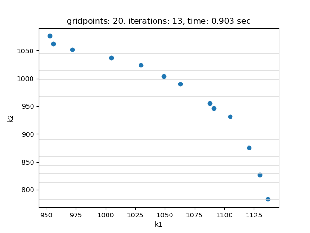
The example is easily scalable by allowing to set the number of items, the number of weight dimensions and the number of objectives through double dash parameters. This example is also part of the GAMS Data Utilities Library, see model [moo01] for reference. The model is solved using EpsConstraint method with 20 gridpoints. The objective function values of the pareto points found are saved in parameter pareto_obj:
----    618 PARAMETER pareto_obj  objective values of the pareto points

                 k1          k2

point1     1137.000     783.000
point2     1130.000     827.000
point3     1121.000     876.000
point4     1105.000     932.000
point5     1091.000     946.000
point6     1088.000     955.000
point7     1063.000     990.000
point8     1049.000    1004.000
point9     1030.000    1024.000
point10    1005.000    1037.000
point11     972.000    1052.000
point12     956.000    1062.000
point13     953.000    1076.000
If plot is set to 1 and Python package matplotlib is installed, a plot of the pareto points is generated:
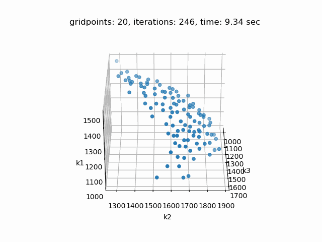
Setting --NBOBJ=3 with model [moo01] allows to solve a knapsack problem with three objectives. These are the resulting pareto points:
Example 2: Solve multi-objective power generation model
The following example demonstrates how to solve a multi-objective power generation model (LP) using the moo LibInclude:
$inlineCom [ ]

$if not set NBOBJ $set NBOBJ  2
$if not set METHOD $set METHOD Sandwiching

Set
   p       'power generation units' / Lignite, Oil, Gas, RES /
   i       'load areas'             / base, middle, peak     /
   pi(p,i) 'availability of unit for load types' / Lignite.(base,middle)
                                                   Oil.(middle,peak), Gas.set.i
                                                   RES.(base, peak)            /
   es(p)   'endogenous sources'  / Lignite, RES /
   k       'objective functions' / cost, CO2emission, endogenous /
   points  'pareto points' / point1*point1000 /;

$set min -1
$set max +1

Parameter dir(k) 'direction of the objective functions 1 for max and -1 for min'
                 / cost %min%, CO2emission %min%, endogenous %max% /
          pareto_obj(points,k) 'objective values of the pareto points';

Set pheader / capacity, cost, CO2emission /;

Table pdata(pheader,p)
                         Lignite    Oil    Gas    RES
   capacity [GWh]          61000  25000  42000  20000
   cost [$/MWh]               30     75     60     90
   CO2emission [t/MWh]      1.44   0.72   0.45      0;

Parameter
   ad        'annual demand in GWh'          / 64000 /
   df(i)     'demand fraction for load type' / base 0.6, middle 0.3, peak 0.1 /
   demand(i) 'demand for load type in GWh';

demand(i) = ad*df(i);

Variable
   z(k)      'objective function variables';

Positive Variable
   x(p,i)    'production level of unit in load area in GWh';

Equation
   objcost   'objective for minimizing cost in K$'
   objco2    'objective for minimizing CO2 emissions in Kt'
   objes     'objective for maximizing endogenous sources in GWh'
   defcap(p) 'capacity constraint'
   defdem(i) 'demand satisfaction';

objcost..   sum(pi(p,i), pdata('cost',p)*x(pi)) =e= z('cost');

objco2..    sum(pi(p,i), pdata('CO2emission',p)*x(pi)) =e= z('CO2emission');

objes..     sum(pi(es,i), x(pi)) =e= z('endogenous');

defcap(p).. sum(pi(p,i), x(pi))  =l= pdata('capacity',p);

defdem(i).. sum(pi(p,i), x(pi))  =g= demand(i);

Model example / all /;

Set kk(k) 'active objective functions';
kk(k) = yes;
$if %NBOBJ%==2 kk('endogenous') = no;

$onEcho > cplex.opt
threads 1
$offEcho

$libInclude moo %METHOD% example LP kk dir z points pareto_obj -iterations=20 -gridpoints=5 -savepoint=1 -savepoint_filename= -savepoint_dir=savepoints -solver=cplex -optfile_init=1 -optfile_main=1
execute 'gdxmerge savepoints%system.DirSep%*.gdx > %system.NullFile%';

display pareto_obj;
This example is also part of the GAMS Data Utilities Library, see model [moo02] for reference. The model is solved using the Sandwiching method with a gap of 0.01 (default). The objective function values of the pareto points found are saved in parameter pareto_obj:
----   1164 PARAMETER pareto_obj  objective values of the pareto points

              cost  CO2emissi~

point1 2112000.000   85824.000
point2 3180000.000   50580.000
point3 4470000.000   20340.000
In addition, savepoint is activated and thus, for each pareto point a point format GDX file that contains information on the solution point will be written. Using gdxmerge all savepoint GDX files can be merged into a single GDX file.
If plot is set to 1 and Python package matplotlib is installed, a plot of the pareto front is generated:
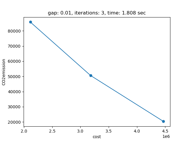
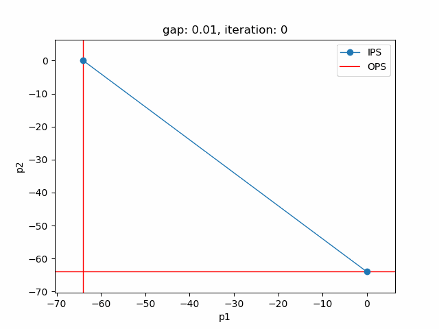
The plot shows the pareto efficient extreme points as well as the lines connecting these points (the IPS). An animation of the algorithm shows how the IPS and OPS are updated at each iteration:
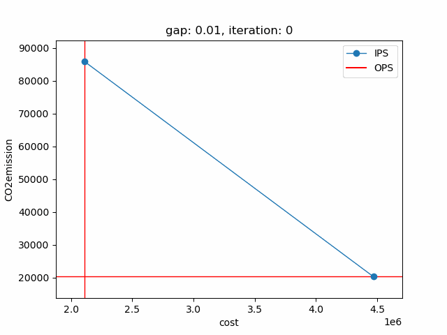
Starting with the initial points from the payoff table, the IPS and the OPS are constructed (iteration 0). In iteration 1, a new point is found and the IPS and OPS are updated. In the last two iterations no new point is found, but the OPS is updated, so the upper bound on the approximation error (distance between the IPS and OPS) decreases and the gap of 0.01 is reached.
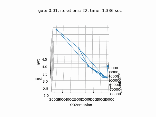
Setting --NBOBJ=3 with model [moo02] allows to solve a power generation problem with three objectives. This is the resulting pareto front:
Example 3: Solve Bensolvehedron model
The following example demonstrates how to solve an instance of Bensolvehedron (LP) using the moo LibInclude:
* number of objectives
$if not set p $set p 2
* complexity of the polyhedron
$if not set m $set m 3

$eval p2m %p%+2*%m%
$eval n (%p2m%)**%p%
$eval n2 2*%n%

Set p               'objectives' / p1*p%p% /
    m               'complexity' / m1*m%m% /
    n2              'variables 2x' / n1*n%n2% /
    n(n2)           'variables' / n1*n%n% /
    cel             'elements in C' / c1*c%p2m% /
    comb(n,p,cel)   'all combinations of elements in C' / system.powerSetRight /
    points          'pareto points' / point1*point1000 /;

Parameter C(p,n)                'objective matrix'
          C_val(cel)            'value of elements in C'
          A(n2,n)               'constraint matrix'
          b(n2)                 'constraint vector'
          dir(p)                'direction of the objective functions 1 for max and -1 for min' / #p -1 /
          pareto_obj(points,p)  'objective values of the pareto points';

A(n,n) = 1;
A(n2,n)$(ord(n2)=ord(n)+card(n)) = -1;
b(n) = 1;
C_val(cel) = ord(cel)-((%p2m%-1)/2)-1;
loop(comb(n,p,cel),
  C(p,n) = C_val(cel);
);

Variable Z(p)           'objective variables';
Positive Variable X(n)  'decision variables';

Equations objectives(p)
          constraints(n2);

objectives(p).. Z(p) =e= sum(n, C(p,n)*X(n));
constraints(n2).. sum(n,A(n2,n)*X(n)) =l= b(n2);

Model bensolvehedron / all /;

$onEcho > cplex.opt
threads 1
$offEcho

$libinclude moo Sandwiching bensolvehedron LP p dir Z points pareto_obj -solver=cplex -optfile_init=1 -optfile_main=1

display pareto_obj;
Bensolvehedron is a class of multi-objective optimization problems introduced on besolve.org. An instance of Bensolvehedron is generated based on the number of objectives p and the complexity of the polyhedron m.
This example is also part of the GAMS Data Utilities Library, see model [moo03] for reference. The model is solved using the Sandwiching method with a gap of 0.01 (default). The objective function values of the pareto points found are saved in parameter pareto_obj:
----   1266 PARAMETER pareto_obj  objective values of the pareto points

                 p1          p2

point1      -64.000         EPS
point2      -63.000      -7.000
point3      -61.000     -15.000
point4      -58.000     -22.000
point5      -55.000     -27.000
point6      -50.000     -34.000
point7      -34.000     -50.000
point8      -27.000     -55.000
point9      -22.000     -58.000
point10     -15.000     -61.000
point11      -7.000     -63.000
point12         EPS     -64.000
If plot is set to 1 and Python package matplotlib is installed, a plot of the pareto front is generated:
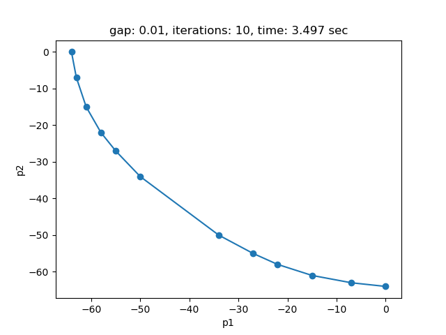
The plot shows the pareto efficient extreme points as well as the lines connecting these points (the IPS). An animation of the algorithm shows how the IPS and OPS are updated at each iteration:
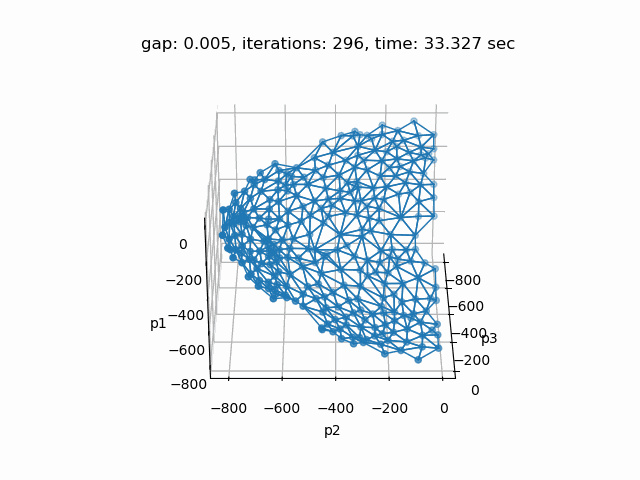
Setting --p=3 with model [moo03] allows to solve the Bensolvehedron problem with three objectives. With a gap of 0.005 the Sandwiching method generates the following pareto front: