Libinclude file rank.gms for ranking one-dimensional numeric data.
Developed by Thomas F. Rutherford, Department of Economics, University of Colorado
Usage:
$libInclude rank v s r [p]
Where:
Type Argument Description Input: v(s) Array of values to be ranked. s A one-dimensional set, the domain of array v. Output: r(s) Rank order of element v(s), an integer between 1 and card(s), ranking from smallest to largest. Optional: (input and output) p(*) On input this vector specifies percentile levels to be computed. On output, it returns the linearly interpolated percentiles.
Note:
rankonly works for numeric data. You cannot sort sets.- The first invocation must be outside of a loop or if block. This routine may be used within a
looporifblock only if it is first initialized with blank invocations ("$libInclude rank"in a context where set and parameter declarations are permitted (See Example 3). - The following names are used within these routines and may not be used in the calling program:
rank_tmp rank_u rank_p
- This routine returns rank values and does not return
sorted vectors, however rank values are easily used to produce a sorted array. This can be done using computed "leads" and "lags" in GAMS' ordered set syntax, as illustrated in examples 1 and 3 below.
Examples
Example 1: Rank a vector, and display the data in sorted order
Set
   i 'Set on which random data are defined'   / a, b, d, c, e, f /
   k 'Ordered set for displaying sorted data' / 1*6 /;

Parameter
   x(i)   'Random data to be sorted'
   r(i)   'Rank values'
   s(k,i) 'Sorted data';

x(i) = uniform(0,1);

$libInclude rank x i r
display x;

* Generate a sorted list using the ordered set k.

* This assignment statement illustrates how the rank orders
* can be used to sort output for display in proper order.  This
* statement uses GAMS support for computed "leads" and "lags"
* on the ordered set k.  The loop is used to improve execution
* speed for larger dimensional sets:

loop(k$sameas(k,"1"),
   s(k+(r(i)-1),i) = x(i);
);

option  s:3:0:1;
display s;
This example is also part of the GAMS Data Utilities Library, see model [rank01] for reference. It writes the following lines to ex1.lst:
----     11 PARAMETER x  Random data to be sorted

a 0.172,    b 0.843,    d 0.550,    c 0.301,    e 0.292,    f 0.224


----     75 PARAMETER s  Sorted data

1.a 0.172
2.f 0.224
3.e 0.292
4.c 0.301
5.d 0.550
6.b 0.843
The rank libinclude can be used to also sort variable levels as the following example shows:
Set
   i 'Set on which random data are defined'   / a, b, d, c, e, f /
   k 'Ordered set for displaying sorted data' / 1*6 /;

Variable
   x(i)   'Random data to be sorted'
Parameter
   r(i)   'Rank values'
   s(k,i) 'Sorted data';

x.l(i) = uniform(0,1);

$onDotL
$libInclude rank x i r
display x.l;

loop(k$sameas(k,"1"),
   s(k+(r(i)-1),i) = x(i);
);

option  s:3:0:1;
display s;
Before the "$libInclude rank" the dollar control option $onDotL needs to be activated.
Example 2: Generate percentiles for a random vector
Set
   i 'Set on which random data are defined' / a, b, d, c, e /
   p 'Percentiles (all of them)'            / 0*100 /;

Parameter x(i) 'Random data to be sorted';

* Generate the random data on set i:
x(i) = uniform(0,1);
display x;

Parameter
   r(i)   'Rank values'
   pct(*) 'Percentiles to be computed' / 20 20.0, median 50.0, 75 75.0 /;

* Generate ranks and compute the specified percentiles (Note that
* the rank array, r, is required, even if the values are not used.)

$libInclude rank x i r pct

* Display three percentiles:
display pct;
This example is also part of the GAMS Data Utilities Library, see model [rank02] for reference. The random data are displayed as follows in the listing file:
----     11 PARAMETER x  Random data to be sorted

a 0.172,    b 0.843,    d 0.550,    c 0.301,    e 0.292
The interpolated percentiles are computed as follows:
----    103 PARAMETER pct  Percentiles

20     0.268,    75     0.550,    median 0.301
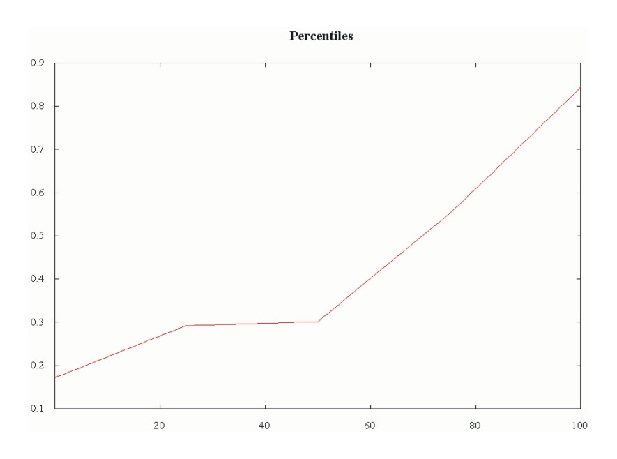
The following code evaluates a full set of percentiles, from 1 to 100. The GAMS special value of EPS is used to represent zero in the percentile calculation. (Percentiles between zero and one are not permitted to avoid misunderstandings about how percentiles are scaled.) The code makes use of Tom Rutherfords plot libInclude available at https://www.mpsge.org/gnuplot/index.html
pct(p) = (ord(p) - 1) + eps;
pct("median") = 0;
display pct;

$libInclude rank x i r pct
display pct;

* Plot the results using GNUPLOT:

Set pl(p) / 20, 40, 60, 80, 100 /;
$setGlobal domain p
$setGlobal labels pl
$libInclude plot pct
This is the generated plot:
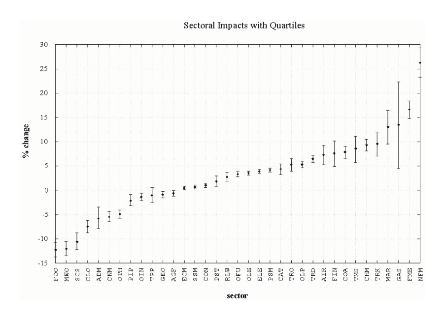
Example 3: Use RANK to report multisectoral Monte Carlo results
One of the most perplexing challenges in economic modeling with GAMS is to present multisectoral results in an easily interpreted format. One simple idea is to present sectoral results in a sorted sequence to make it easier to identify the most seriously affected sectors. The presentation of results in a multisectoral model is made even more challenging when model results are generated for a randomized set of scenarios. A summary of Monte Carlo results involves reporting both mean results and their sensitivity. One means of characterizing the sensitivity of model results is to report functions of the sample distribution such as the upper and lower quartiles.
This example illustrates how rank can be used to help report results from the Monte Carlo analysis of a multisectoral model.
The complete model used as example here is part of the GAMS Data Utilities Library, see model [rank03] for reference. The following extract of that model generates the result we want to look at.
* Determine ranking of sectors by mean impact:
mean(i) = qvalue(i,"mean");
$libInclude rank mean i meanrank

* The following statement creates a tuple matching the ordered
* set, ki, to the set of sectors, i.  In this tuple, the sequence of
* assignments corresponds to increasing mean impacts:
imap(ki+(meanrank(i)-ord(ki)),i) = yes;

* Evaluate quartiles of sectoral impacts for each sector:
loop(i,
   x(s) = v(s,i);

*  Load quartile with the percentiles to be
*  evaluated (25th, 50th and 75th):
   quartile(qtl) = qv(qtl);

$  libInclude rank x s r quartile

*  Save the quartile values:
   qvalue(i,qtl) = quartile(qtl);
);
display qvalue;

Parameter results(ki,i,*) 'Summary of impacts (sorted)';
results(ki,i,"mean")$imap(ki,i) = mean(i);
results(ki,i,qtl)$imap(ki,i)    = qvalue(i,qtl);
display results;
The program produces the following display output:
               q25         q50         q75        mean

1 .FOO     -13.767     -12.110     -10.671     -12.259
2 .MWO     -13.496     -11.982     -10.512     -12.035
3 .SCS     -12.244     -10.418      -8.738     -10.588
4 .CLO      -8.763      -7.407      -6.158      -7.480
5 .ADM      -7.865      -5.601      -3.470      -5.812
6 .CNM      -6.437      -5.320      -4.404      -5.461
7 .OTH      -5.732      -4.781      -4.012      -4.892
8 .PIP      -3.142      -1.930      -0.836      -2.145
9 .OIN      -2.124      -1.339      -0.563      -1.358
10.TPP      -2.527      -0.988       0.521      -1.041
11.GEO      -1.542      -0.826      -0.196      -0.883
12.AGF      -1.178      -0.624      -0.072      -0.625
13.ECM       0.137       0.466       0.796       0.441
14.SSM       0.303       0.711       1.079       0.684
15.CON       0.604       1.071       1.479       1.041
16.PST       0.814       1.924       2.966       1.858
17.RLW       1.885       2.787       3.632       2.738
18.OFU       2.789       3.300       3.829       3.330
19.OLE       3.155       3.553       3.964       3.554
20.ELE       3.480       3.896       4.318       3.892
21.PSM       3.733       4.134       4.591       4.168
22.CAT       3.216       4.417       5.461       4.369
23.TRO       3.953       5.123       6.549       5.282
24.OLP       4.614       5.262       5.909       5.295
25.TRD       5.694       6.454       7.250       6.476
26.AIR       5.227       7.182       9.276       7.320
27.FIN       4.919       7.301      10.175       7.640
28.COA       6.581       7.818       9.125       7.878
29.TMS       5.668       8.530      11.086       8.591
30.CHM       8.071       9.299      10.534       9.319
31.TRK       7.031       9.367      11.851       9.577
32.MAR       9.485      13.072      16.424      13.049
33.GAS       4.437      13.183      22.311      13.462
34.FME      14.794      16.617      18.382      16.642
35.NFM      23.299      26.398      29.281      26.263
The tabular report is helpful, but it does not convey the results as immediately as a picture. GNUPLOT's errorbar plot format is a convenient graphical format for portraying this information. The libinclude interface to GNUPLOT does not support this type of plot, so the continuation of the program produces the GNUPLOT command and data files before invoking the GNUPLOT program:
* Write out a GNUPLOT file to generate a chart of the results:

File kplt / ex3.gnu /;
put  kplt;
kplt.lw = 0;

put "reset"/;
put 'set title "Sectoral Impacts with Quartiles"'/;
put "set linestyle 1 lt 8 lw 1 pt 8 ps 0.5"/;
put "set grid"/;
put 'set ylabel "% change"'/;
put "set xzeroaxis"/;
put "set bmargin 4"/;
put "set xlabel 'sector'"/;
put 'set xrange [1:',card(i),']'/;
put 'set xtics rotate (';
loop(ki, loop(i$imap(ki,i), put '\'/' "',i.tl,'" ', ord(ki):0,',';));
put @(file.cc-1) ')'/;
put "plot 'ex3.dat' notitle with errorbars ls 1"/;
putClose;

File kpltdata / ex3.dat /;
put  kpltdata;
kpltdata.nr =  2;
kpltdata.nw = 14;
kpltdata.nd =  6;
loop(ki, loop(i$imap(ki,i), put ord(ki):0,qvalue(i,"mean"), qvalue(i,"q25"), qvalue(i,"q75")/;));
putClose;
execute 'wgnupl32 ex3.gnu -';
This is the generated plot:
Example 4: Repeated computation of percentiles within a loop
The following code extract shows how to do repeated computation of percentiles within a loop while the data is changing. This is an extract of the model [rank04] from the GAMS Data Utilities Library.
* Do several iterations, computing percentiles in each step:

loop(iter,
*  Substitute a call to the NLP solver by a call to the random
*  number generator.  In many applications, this substitution
*  produces profoundly more sensible results.
*
*  solve catchment using nlp maximizing max;

   z(week) = uniform(0,1);

*  If you want to retrieve percentile values, you need to reassign
*  the percentiles that you wish to retrieve at this point in the
*  program.  If pct() were not reassigned at this point, the INPUT
*  values would correspond to the OUTPUTs from the previous call.

   pct(pctl) = pct0(pctl);

$  libInclude rank z week rnk pct

   pctval(iter,pctl) = pct(pctl);
);

display pctval;
Output:
----     58 Here are the INPUT values of PCT0 and PCT prior to the call to rank:

----     58 PARAMETER pct0  Percentiles to be computed

50 50.000,    75 75.000,    80 80.000,    95 95.000


----     58 PARAMETER pct  Percentiles to be computed (input) and those values (output)

50 50.000,    75 75.000,    80 80.000,    95 95.000


----    153 Here are the values of PCT0 and PCT after the call to rank:

----    153 PARAMETER pct0  Percentiles to be computed

50 50.000,    75 75.000,    80 80.000,    95 95.000


----    153 Note that rank has changed the OUTPUT value of pct

----    153 PARAMETER pct  Percentiles to be computed (input) and those values (output)

50 0.424,    75 0.662,    80 0.712,    95 0.864


----    273 PARAMETER pctval  Percentile values in successive iterations

                50          75          80          95

iter1        0.345       0.594       0.638       0.922
iter2        0.385       0.633       0.672       0.941
iter3        0.474       0.705       0.766       0.962
iter4        0.627       0.796       0.823       0.978
iter5        0.428       0.682       0.793       0.904
iter6        0.422       0.690       0.729       0.958
iter7        0.558       0.716       0.756       0.902
iter8        0.451       0.638       0.726       0.942
iter9        0.464       0.704       0.755       0.916
iter10       0.564       0.805       0.831       0.974
Example 5: Generating percentiles for heterogenous households.
$title Percentile ranking of household expenditure data with heterogenous household size

Set h / 0*100 /;

Parameter
   y(h)    'Aggregate expenditure associated with household type h'
   n(h)    'Number of persons associated with household type h'
   ypc(h)  'Per-capita expenditure of household type h'
   rank(h) 'Rank of household in per-capita expenditure';

* Assign some random values:
y(h)   = uniform(0.2,1.2);
n(h)   = uniform(1,6);
ypc(h) = y(h)/n(h);

* Assign ranks to household based on per-capita expenditures:
$libInclude rank ypc h rank

* Now determine percentile ranking of the households taking into account
* differences in numbers of members and household representation:
Set r 'Temporary set used for ranking' / r0*r100 /;

Parameter
   pcttmp(r) 'Temporary array for computing percentiles'
   pct(h)    'Percentile rankings for households';

Set r0(r) / r0 /;

* First, create an array with households assigned
loop((r0(r),h), pcttmp(r+(rank(h)-1)) = n(h););
loop(r,         pcttmp(r) = pcttmp(r) + pcttmp(r-1););
pcttmp(r) = pcttmp(r)/sum(h, n(h));

loop((r0(r),h), pct(h) = pcttmp(r+(rank(h)-1)););

Parameter ranking 'Ranking of households and expenditures';

loop((r0(r),h),
   ranking(r+(rank(h)-1),h,"n")   = n(h);
   ranking(r+(rank(h)-1),h,"ypc") = ypc(h);
   ranking(r+(rank(h)-1),h,"pct") = pct(h);
);

display ranking;
This example is also part of the GAMS Data Utilities Library, see model [rank05] for reference. It produces the following output:
                         n         ypc         pct
        r0  .43        5.662       0.044       0.018
        r1  .8         5.682       0.047       0.036
        r2  .58        4.477       0.052       0.050
        r3  .14        5.742       0.058       0.068
        r4  .55        4.815       0.063       0.083
        r5  .65        3.702       0.063       0.094
        r6  .61        5.880       0.064       0.113
        r7  .54        4.463       0.064       0.127
        ....
        r98 .62        1.134       0.640       0.991
        r99 .10        1.673       0.716       0.997
        r100.73        1.053       1.076       1.000