Table of Contents
- Some Basic Economic Ideas
- Specifying an MPSGE Model
- An Introductory Example: Two Goods and Two Factors in a Closed Economy
- Modeling Intermediate Demand and Joint Production
- Modeling a Small Open Economy
- MPSGE Keywords and Syntax
- MPSGE-Specific Output
- Appendix
MPSGE is a language used for formulating and solving Arrow–Debreu economic equilibrium models and exists as a subsystem within GAMS. The name stands for ‘mathematical programming system for general equilibrium’. MPSGE provides a short-hand non-algebraic representation for the systems of nonlinear inequalities which underly general equilibrium models. The MPSGE framework is based on nested constant elasticity of substitution utility and production functions. The data requirements for a model include share and elasticity parameters, endowments, and tax rates for all the consumers and production sectors in the model. These may or may not be calibrated from a consistent benchmark equilibrium dataset.
The main benefit of using MPSGE is that modelers are released from having to write the equations of the model and the calibrated demand and supply functions. Experience shows that even computing the parameters of the functions is error-prone. The tabular input format of MPSGE facilitates a compact, non-algebraic representation of the equations of a model. Thus algebraic tedium and the scope for programming errors are reduced, and more attention can be paid to economic interpretation and testing of alternative formulations.
This chapter offers an introduction to MPSGE for users who are familiar with GAMS. For more information on MPSGE and details on more advanced features, see [156] and [130]. In addition, a library of small examples for self-study is available here .
This chapter is organized as follows. We start with an overview of some basic economic ideas and general remarks on specifying an MPSGE model. Next, we introduce a first simple example. Then we demonstrate how intermediate demand and joint production are modeled with MPSGE. We follow with a third model that features a small open economy and also includes taxes on inputs and outputs, labor-leisure choice, classical unemployment, and nested demand functions. We conclude the chapter with an overview of MPSGE keywords and the syntax for specifying functions, some other features like domain restrictions on variable declarations, and a few brief comments on MPSGE-specific output in the GAMS listing file. Note that a full version of all MPSGE models that are discussed, including standard GAMS versions, are given in the Appendix.
Some Basic Economic Ideas
MPSGE models are based on the following economic ideas. In each model there are multiple interacting agents, where each agent solves an optimization problem. For example, consumers maximize utility subject to their budget constraint, and producers minimize their cost given available technology. Agent interactions are mediated by markets and prices and the optimal solution is an equilibrium where prices and activity levels have adjusted so that markets for produced goods and input factors clear. In equilibrium, each agent cannot do better by altering their behavior (given the constraints they face). In this section we give more details on these basic economic ideas. In particular, we offer brief introductions to consumer demand theory, producer supply theory and general economic equilibrium.
Consumer Demand Theory
Consumer choice is modeled using an optimization paradigm: consumers form a consumption bundle which maximizes welfare subject to a budget constraint. As an abstract notion, this seems plausible, but certain details must be dealt with to provide an operational application of the idea.
Consider the following example. Thomas lives in Ann Arbor where he spends 30% on housing and the rest of his income on other goods. This information is essentially an observation of a benchmark equilibrium, consisting of the prevailing prices and quantities of goods demanded. Now, Thomas has an employment offer in Berlin which pays 50% more than he currently earns, but he is hesitant to take the job since rental rates in Berlin are three times higher than in Ann Arbor. The question is: On purely economic grounds, should he move?
Thomas' choices are illustrated below. Point \(a\) represents the benchmark point, where he spends the amount \(H_a\) on housing in Ann Arbor. Point \(b\) represents a potential trade-off between housing and other goods in Berlin, where he spends a lower percentage of his income on housing and more on other goods.

Whether Thomas derives the same welfare from the choices represented by point \(b\) like those represented by point \(a\) depends on the elasticity of substitution. The elasticity of substitution is the willingness to exchange some amount of one good for more of the other good. The three curves in the figure above represent three elasticities of substitution. Note that the less convex (flatter) the curve is, the higher is the elasticity, i.e. the more willing is Thomas to substitue housing for other goods.
If the elasticity of substitution equals \(\sigma^{\star}\), Thomas is indifferent between choices \(a\) and \(b\), since both points lie on the respective indifference curve. However, if the elasticity of substitution is lower, say is equals \(\sigma_L\), or higher, say it equals \(\sigma_H\), then \(b\) will be worse than \(a\) and Thomas will not choose it. Hence, the elasticity of substitution is crucial in determining whether Thomas should move on economic grounds. Note that the elasticity of substitution is a measure for Thomas' preferences.
The utility function can be deduced if prices and the associated choices are observed and the elasticity of substitution is given. Thus, in MPSGE, a utility function is represented by benchmark (or observed) quantities, benchmark prices and the associated elasticity of substitution. Benchmark quantities determine an anchor point for the set of indifference curves. Benchmark prices fix the slope of the indifference curve at that point. The elasticity of substitution is a measure of the curvature of the indifference curve and specifies the utility function unambiguously.
Producer Supply Theory
While consumers aim to maximize their utility subject to a budget, producers aim to reduce their cost of production given available technology. The activity of a firm is modeled as a production function that maps inputs into outputs. Inputs are primary factors like labor, capital, land, raw materials etc. and outputs are goods and services. Similarly to utility functions, in MPSGE, a production function is represented by reference quantities of reference prices of inputs and outputs, elasticities of substitution and elasticities of transformation.
Summarizing, the main principle for both, consumers and producers, is choice. Consumers choose quantities of goods given their preferences, prices and budgets. Producers choose quantities of primary factors and output levels given available technology. Available technology is modeled via elasticities of substitution between inputs and elasticities of transformation between outputs.
General Economic Equilibrium
As mentioned above, MPSGE is a system for modeling general economic equilibria. General economic equilibrium analysis studies the working of an economic system as a whole. The basic assumption is that there are two types of agents in the economy: producers and consumers. Producers are assumed to operate with constant return to scale and to be perfectly competitive price-taking firms. Further, they are assumed to select factor inputs and output levels in order to maximize their profits given available technology. Consumers are assumed to maximize their welfare subject to budget constraints (incomes and endowments). An economy is in economic equilibrium if all consumers spend their given incomes such that they gain maximum satisfaction, all firms in each sector minimize their costs given availabe technology, and prices (for primary factors and commodities) and activity levels have adjusted such that all agents cannot do better by altering their behavior given the constraints they face. In equilibrium, all markets have cleared: in both, goods and factors markets, total demand equals total supply.
Mathematically, such an economy is modeled as a system of weak inequalities, where each inequality is associated with a non-negative variable denoting a price or a quantity. If a particular weak inequality holds as an equation, then the associated variable is strictly positive. If it holds as a strict inequality, then the associated variable equals zero. This is a mixed complementarity problem that can be formulated and solved with standard GAMS syntax. For details see section Mixed Complementarity Problems (MCPs). As we will demonstrate, MPSGE models can be translated to standard GAMS MCP models. However, the framework that MPSGE offers is much more user-friendly, since modelers do not have to input the complex equations manually.
Specifying an MPSGE Model
In this section we give an overview of the MPSGE model specification, a simple introductory example follows in the next section. Like any standard GAMS program, a program with an embedded MPSGE model begins with set and parameter definitions that will later be used in the model. The MPSGE model is specified within an $ontext / $offtext block.
First, the name of the model must be defined:
$MODEL:mymodel
Here $MODEL is an MPSGE keyword and the model name mymodel is a GAMS identifier.
In a GAMS program lines within $on/offtext are are treated as a block comment. However, if the preprocessor encounters the MPSGE model definition statement, it will recognize that an MPSGE model specification follows and will process the code accordingly.
- Note
- Like GAMS, MPSGE is not case sensitive.
Secondly, the variables for an MPSGE model are declared. In every model, there are three classes central variables:
$SECTORS:variables for activity levels associated with constant returns to scale production sectors in the economy, which are non-negative,$COMMODITIES:variables for commodity prices including all final goods, intermediate goods and primary factors of production, which are also non-negative, and$CONSUMERS:variables for income levels, one for each “household” in the model, including any government entities.
In addition, models may include auxiliary variables ($AUXILIARY) that are used to introduce endogenous tax instruments or endogenous endowment quantities to a model.
- Note
- Unlike GAMS models, variables in an MPSGE model must be declared over an explicit domain. Only variables that have been declared as one of the four MPSGE variable types may be used in the MPSGE model. Error messages are generated for variables which are declared but not referenced.
Thirdly, the parameters for functions are specified in a structured manner. The general syntax for all possible entries is given is section Syntax for Production and Demand Functions below. The MPSGE framework uses these specifications to automatically generate the respective market-clearing and income-balance equations. There are two types of functions:
$PROD:This block defines a production function, specifying inputs, outputs and elasticities of substitution and transformation. A production function must be given for each sector in the model. Note that most of the power and subtleties of the MPSGE framework center on the$PRODtables.$DEMAND:This block defines a demand function. This function represents preferences (using reference demands), initial factor endowments and elasticities of substitution. A demand function must be specified for each consumer in the model.
Finally, any auxiliary variable has an associated equilibrium condition that is defined by the user with conventional GAMS algebraic syntax and placed in a block called $CONSTRAINT.
These four parts - model definition, variable declarations, function specifications and possibly side constraints for auxiliary variables - are the core of the MPSGE model specification. The model specification is followed by the dollar control option $offtext and the following compiler directive:
$sysinclude mpsgeset mymodel
This compiler directive instructs MPSGE to compile the functions and generates an external file called MYMODEL.GEN. This external file is then loaded to the GAMS file with the following directive:
$include MYMODEL.GEN
Finally, a standard GAMS solve statement follows and the model will be handed for solution to one of the MCP solvers:
solve mymodel using mcp;
Observe that the appropriate GAMS model type is MCP.
Most often the model is first evaluated at the benchmark point to test whether it is properly calibrated and everything works as expected. This is achieved by setting the option iterlim to zero. Then one or more counterfactuals are solved: first some parameter is modified using standard GAMS syntax, then the $include statement is repeated and the model is solved again.
- Note
"$sysInclude mpsgeset"allows for an optional argument-mt=0or1after the model name. The default value for the argumentmtcan be controlled via the double dash option--MPSGEMT=0or1. If themtoption is set to 1 theMODEL.GENfile is created in the GAMS scratch directory. Hence the$includebefore the solve needs to read$include "%gams.scrdir%MODEL.GEN". This allows to run multiple MPSGE jobs with the same model in the same working directory. The default of this option is 0. The model hansmge demonstrates the use.
An Introductory Example: Two Goods and Two Factors in a Closed Economy
In the canonical 2x2 model, two final goods, \(X\) and \(Y\), are produced with two primary factors, labor \(L\) and capital \(K\), and there is a single representative agent (consumer) \(RA\). The model is defined by technology, preferences and endowments. We can describe preferences by a utility function which provides an ordinal ranking of consumption levels for \(X\) and \(Y\). We assume that both factors are in fixed supply, thus in equilibrium, factor endowments equal factor demands, and the supply of the two goods equal their demand.
The problem can be cast as consisting of three production activities, \(X\), \(Y\) and \(U\), and five markets \(X\), \(Y\), \(U\), \(K\) and \(L\). The initial data for the model are given by the following matrix.
                 Production Sectors     Consumers
                 ----------------------------------
    Markets       X      Y      U         RA         Row Sums
    ---------------------------------------------------------
    PX           100          -100                     0
    PY                   50    -50                     0
    PU                         150       -150          0
    PK           -50    -20                70          0
    PL           -50    -30                80          0
    ---------------------------------------------------------
    Column Sums    0      0      0          0
    ---------------------------------------------------------
The data describes a representative equilibrium. Rows correspond to markets, where \(PX\), \(PY\), \(PU\), \(PK\) and \(PL\) are the prices for the commodity \(X\), the commodity \(Y\), the utility \(U\), and capital and labor respectively. Positive entries denote the value of commodity flows into the economy (sales or factor supplies) and negative entries represent the value of commodity flows out of the economy (factor demands and good demands). Observe that the sum of a row will equal zero if the market clears, i.e. the total amount of commodity that flows into the economy equals the total amount of this commodity that flows out of the economy. The matrix is called balanced if all rows and columns sum to zero.
Note that the layout of the matrix ensures that a complete list of the transactions associated with an activity is given in each production column. The sum of a production sector column is zero if the value of the outputs equals the costs of the inputs. A consumer column is balanced if the sum of primary factor sales equals the value of final demands. Hence columns that sum to zero indicate zero profits. This type of matrix is related to the concept of a social accounting matrix (or short: SAM).
The problem can be modeled with GAMS MPSGE as follows:
Parameter   endow     index of labour endowment     / 1.0 /;

*       MPSGE model declaration follows

$ontext
$MODEL:twobytwo

$SECTORS:
    X   ! Activity level for sector X -- benchmark=1
    Y   ! Activity level for sector Y -- benchmark=1
    U   ! Activity level for sector U -- benchmark=1

$COMMODITIES:
    PX  ! Relative price index for commodity X -- benchmark=1
    PY  ! Relative price index for commodity Y -- benchmark=1
    PU  ! Relative price index for commodity U -- benchmark=1
    PL  ! Relative price index for labor -- benchmark=1
    PK  ! Relative price index for capital -- benchmark=1

$CONSUMERS:
    RA  ! Income level for representative agent -- benchmark=150;

$PROD:X s:1
        O:PX   Q:100
        I:PL   Q: 50    ! Variable LX in the algebraic model
        I:PK   Q: 50    ! Variable KX in the algebraic model

$PROD:Y s:1
        O:PY   Q: 50
        I:PL   Q: 20    ! Variable LY in the algebraic model
        I:PK   Q: 30    ! Variable KY in the algebraic model

$PROD:U s:1
        O:PU   Q:150
        I:PX   Q:100    ! Variable DX in the algebraic model
        I:PY   Q: 50    ! Variable DY in the algebraic model

$DEMAND:RA
        D:PU
        E:PL   Q: (70*endow)
        E:PK   Q: 80

$offtext

* Compiler directive instructing MPSGE to compile the functions

$sysinclude mpsgeset twobytwo

* Benchmark replication

twobytwo.iterlim = 0;
$include TWOBYTWO.GEN
solve twobytwo using mcp;
abort$(abs(twobytwo.objval) gt 1e-7) "*** twobytwo does not calibrate ! ***";
twobytwo.iterlim = 1000;

*   Counterfactual : 10% increase in labor endowment

endow = 1.1;

*   Solve the model with the default normalization of prices which
*   fixes the income level of the representative agent.  The RA
*   income level at the initial prices equals 80 + 1.1*70 = 157.

$include TWOBYTWO.GEN
solve twobytwo using mcp;
Note that an algebraic version of this model using standard GAMS syntax is given in the Appendix.
After the model statement where the model is named, variables are declared in each of the three central variable classes. Unlike conventional GAMS syntax, in MPSGE, trailing comments in variable declarations (starting with the symbol !) are interpreted as variable descriptors that will appear in the listing file.
Then three production blocks $PROD - one for each sector - follow. Output parameters are specified in the line starting with the label O and input parameters are given in the line starting with the label I, the respective quantities are listed in the field Q. Note that the first input in the production block for sector X represents labor demand in sector X and the second input represents capital demand in sector X. Similarly, the inputs in the production block for sector Y represent labor and capital demand for sector Y. In the production block for sector U, the inputs represent demand for X and Y in sector U. In the field s: next to the name of the sector the elasticity of substitution between the inpiuts is specified.
A demand block $DEMAND for the consumer RA completes the model specification. Demand parameters are specified in the line starting with the label D and endowment parameters are given in the line starting with the label E . Note that all possible entries for production and demand blocks are discussed in section Syntax for Production and Demand Functions. Observe that there is no algebraic formulation of equations, only parameter specifications. Given this input, the MPGSGE framework generates the respective equations automatically.
Note that it is not necessary to fix a numeraire. If a numeraire is not specified, the normalization of prices is arbitrary. For example, in the model above, RA is used as a numeraire and the following remark appears in the listing file:
Default price normalization using income for RA
Note that the version of this model in the Appendix includes two additional counterfactual scenarios, where first sector X is used as numeraire commodity and then the wage rate PL is fixed as numeraire. In the Appendix, there are also two alternative versions of the model above: a model in standard GAMS syntax where the equations that are automatically generated by the MPSGE framework are given explicitly, and an MPSGE model that uses vector notation instead of scalars.
Modeling Intermediate Demand and Joint Production
In this section we extend the two by two model above in the following three ways:
- We distinguish between production sectors and produced goods.
- Each sector produces both goods, so we have joint production.
- In addition to primary factors like labor and capital, goods enter the production process as inputs. Thus we have intermediate demand.
The full MPSGE model and MCP and NLP versions of the model are given in the Appendix. Here we reproduce and discuss only selected code snippets. The main difference to the simple model above is the specification of the production block:
$PROD:X(j)   s:1    t:1
      O:P(i)    Q:make0(i,j)    ! S(i,j) in the MCP and NLP models
      I:P(i)    Q:use0(i,j)     ! D(i,j) in the MCP and NLP models
      I:PF(f)   Q:fd0(f,j)      ! FD(f,j) in the MCP and NLP models
Note that the supply is specified in the output line, the intermediate demand is given in the first input line and the factor demand is listed in the second input line. Thus each sector j produces the goods i using the intermediate goods i and the primary factors f. Consider the fully spelled-out production block for sector s1:
$PROD:X("s1")   s:1    t:1
      O:P("g1")        Q:6.0
      O:P("g2")        Q:2.0
      I:P("g1")        Q:4.0
      I:P("g2")        Q:2.0
      I:PF("labor")    Q:1.0
      I:PF("capital")  Q:1.0
At benchmark, sector s1 produces 6 units of good g1 and 2 units of good g2. The input for this output is 4 units of the good g1, 2 units of the good g2 and labor (one unit) and capital (one unit).
- Note
- Double quotes have to be used if a singleton set element is referenced in an MPSGE model. Single quotes are not recognized.
Observe that the technology used to combine these four production factors is based on a Cobb-Douglas production function, i.e. the elasticity of substitution equals 1, as indicated by the value in field s. In addition, the curvature of the production possibility frontier (the constant elasticity of transformation function) is given in field t.
Modeling a Small Open Economy
An open economy is one in which goods are traded on international markets, typically at fixed international prices, i.e. there are imports and exports. One class of models for small open economies are known as "123 models" [41]. In the original 123 model, there was one small country, two producing sectors and three goods (one domestic good, one import good and one export good). The 123 model we present and discuss in this section has exogenously given world prices for imports and exports, taxes, labor-leisure choice, classical unemployment and joint production. The programming language keeps track of tax revenue flows, equations which are otherwise tedious to program. The model is a tiny version of the open economy GTAP model [115]. It follows the canonical microeconomic optimization framework: (i) consumers maximize welfare subject to a budget constraint with fixed levels of investment and public expenditure, and (ii) producers combine intermediate inputs and primary factors at least cost for given technology.
Note that the full MPSGE model mge123 and an algebraic version are given in the Appendix. In addition, we introduce and discuss a version of the model that includes nesting. Note further, that the data for the model and its variants are included in a separate GAMS file. Observe that the input-output matrix in the data file provides data on value flows for primary production factors, intermediate goods and final consumption products. In the following, we comment on selected code snippets and thereby discuss the most important features of the model.
Consider the production block for the entire production of the small economy:
$PROD:Y  t:etadx s:esubkl
        O:PD    Q:d0    P:1                             ! YD
        O:PX    Q:x0    P:px0   A:GOVT  T:tx            ! YX
        I:RK    Q:kd0   P:rr0   A:GOVT  T:tk            ! KD
        I:PL    Q:ly0   P:pl0   A:GOVT  T:tl N:TAU_TL   ! LY
Note that the first output line represents production for the domestic market, which is denoted by the variable YD in the algebraic version of the model. The reference price at benchmark is given in the new field P.
- Note
- The default value for both P and Q fields is 1.0
The second output line represents production for the export market (variable YX in the algebraic version). Observe that taxes are specified in the two new fields A and T: the tax recipient is specified in field A and the tax rate is listed in field T. Note that the tax recipient must reference a $CONSUMER variable and the tax rate tx (tax rate on exports) is given exogenously.
- Attention
- In MPSGE, the way exogenous taxes are computed depends on whether they are imposed on outputs or inputs. Taxes on outputs are specified on a gross basis. Hence, if a tax on outputs has proportional rate \(t\), the producer price will be \(p(1-t)\), where \(p\) is the market price. However, taxes on inputs are specified on a net basis. Hence, if a tax on inputs has ad valorem rate \(t\) , the user cost will be \(p(1+t)\), where \(p\) is the market price.
The first input line represents capital demand (variable KD in the algebraic version). The model includes investment by the private (domestic) households, thus the variable RK denotes a rental price index. Observe that capital is taxed exogenously at the capital tax rate tk.
The second input line represents labor demand (variable LY in the algebraic version). In addition to an exogenous labor tax tl, an endogenous tax is imposed on this input. The endogenous tax rate is determined by the auxiliary variable TAU_TL, which is the entry in the field N at the end of the line. Note that an equation associated with the auxiliary variable is specified in the following block:
$CONSTRAINT:TAU_TL
        GOVT =e= PA * g0;
- Note
- When an auxiliary variable is fixed no constraint is required. When the lower bound of the auxiliary variable is less than the upper bound, a constraint is required.
Note further, that the variable TAU_TL is a wage replacement tax and at benchmark, it is fixed at zero. It is positive in two of the four counterfactual scenarios.
Domestic demand is modeled using the Armington assumption: consumers demand one single good which is an aggregation of composite goods consisting of the goods produced domestically and the imported versions, where imports and domestic goods in the same sector are imperfect substitutes. The aggregated composite good is given by a constant elasticity of substitution aggregation function of the domestic goods and the imported goods with elasticity of substitution sigmadm. In our model, sigmadm equals 4 (domestic versus imported goods). The production of the Armington good is specified in the following block:
$PROD:A  s:sigmadm
        O:PA    Q:a0    A:GOVT  t:ta
        I:PD    Q:d0                        ! DA
        I:PM    Q:m0    p:pm0 A:GOVT t:tm   ! MA
Note that both inputs are intermediate goods. The first input line represents domestic absorption (variable DA in the algebraic version of the model) and the second input line represents imports (variable MA in the algebraic version). Imports are taxed with the import tariff rate tm and the composite good is taxed with the excise and sales tax rate ta. Both taxes are exogenous.
In addition, the model contains production blocks for imports and exports. Foreign exchange (denoted by the MPSGE variable PFX) is used in these two production blocks. It is the input in the production block for imports and the output in the production block for exports.
The two consumers in the model are the government (MPSGE variable GOVT) and aggregated private households (MPSGE variable HH). The demand block for the government agent is as follows:
$DEMAND:GOVT
        E:PFX   Q:bopdef
        E:PA    Q:dtax
        E:PA    Q:g0            R:TAU_LS
        D:PA
Note that the first endowment line represents the balance of payment in the current account (denoted by the $COMMODITIES variable PFX). In our model, exports exceed imports resulting in the deficit bopdef. If imports are larger than exports there will be a surplus. The other two endowment lines represent taxes that are paid by the households: a direct tax dtax and a lumpsum labor replacement tax that is specified as an auxiliary variable and determined by the respective complementarity equation. In this model the labor replacement tax is either a lumpsum tax (TAU_LS) or it is levied on labor at a tax rate of TAU_TL (see above). Note that the direct tax and the lumpsum tax feature in the demand block for HH as negative endowments. Negative endowments represent payments to be made. The demand block for HH follows:
$DEMAND:HH  s:sigma
        E:PA    Q:(-g0)         R:TAU_LS
        E:PA    Q:(-dtax)
        E:RK    Q:kd0
        E:PA    Q:(-i0)
        E:PL    Q:(ly0+l0)      ! Labor endowment = ly0+l0 - UR * (ly0+l0)
        E:PL    Q:(-(ly0+l0))   R:UR
        D:PA    Q:c0
        D:PL    Q:l0
Households demand two goods: the Armington composite good PA (first demand line) and leisure (second demand line). Note that the first two endowment lines represent taxes as discussed above. The third and fourth endowment line relate to capital: the third line represents the income generated by capital investment and the fourth line represents capital investments. The last two endowment lines refer to labor. Labor endowment for the aggregated households equals the sum of labor and leisure minus the percentage of unemployment. Note that at benchmark, the unemployment rate UG is fixed at zero, other scenarios are explored in the counterfactuals.
In model mge123, the rate of substitution for domestic and imported goods that constitute the Armington good PA is fixed at sigmadm = 4. Suppose that we want more control over substitution possibilities. For example, we may wish to model a substitution rate in final demand that is different than for other uses of the Armington good. MPSGE facilitates modeling this additional degree of freedom through nesting. Consider the following demand block for HH from model mgenested, a variant of model mge123:
$DEMAND:HH  s:sigma    c:sigmac
        E:PA    Q:(-g0)         R:TAU_LS
        E:PA    Q:(-dtax)
        E:RK    Q:kd0
        E:PA    Q:(-i0)
        E:PL    Q:(ly0+l0)          ! Labor endowment = ly0+l0 - UR * (ly0+l0)
        E:PL    Q:(-(ly0+l0))   R:UR
        D:PD    Q:cd0   c:
        D:PM    Q:cm0   c:
        D:PL    Q:l0
Note that in this formulation the endowment lines are unchanged and we have three demand lines. The first two demand lines have an additional field (c:). This tag indicates that these two goods are part of a nest: they are combined to an intermediate good called C. The rate of substitution for the goods in the nest is given in the first line of the demand block: c:sigmac. Observe that except for the substitution rate, C equals PA. The structure of the final demand can be presented graphically using the following nesting diagram:
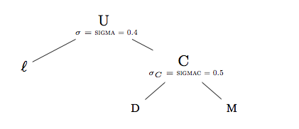
The nested utility function, expressed as a unit function is:
\begin{equation*} U = \left[ \theta \left( \frac{\ell}{\bar \ell} \right)^{1-1/\sigma} + (1-\theta) \left( \alpha \left( \frac{D}{\bar D} \right)^{1-1/{\sigma_C}} + (1-\alpha) \left( \frac{M}{\bar M} \right)^{1-1/{\sigma_C}} \right)^{\frac{1-1/\sigma}{1-1/\sigma_C}} \right]^{1/1-1/\sigma} \end{equation*}
in which \(\theta\) is the budget share of leisure ( \(\ell\)) in aggregate expenditure, and \(\alpha\) is the budget share of domestic goods ( \(D\)) in commodity expenditure, both evaluated at the benchmark point:
\begin{equation*} \theta = \frac{\bar \ell}{\bar \ell + \bar D + \bar M} \end{equation*}
and
\begin{equation*} \alpha = \frac{\bar D}{\bar D + \bar M} \end{equation*}
The demand for leisure is a function of extended income ( \(HH\)):
\begin{equation*} \ell = \bar \ell \left( \frac{p_U}{p_\ell} \right)^\sigma \frac{HH}{p_U \left(\bar \ell + \bar D + \bar M\ \right)} \end{equation*}
The demand for domestic and imported goods is a function of both the top-level elasticity of substitution, \(\sigma\), as well as the elasticity of substitution between consumption goods, \(\sigma_C\):
\begin{equation*} D = \bar D \left( \frac{p_U}{p_C} \right)^\sigma \left( \frac{p_C}{p_D} \right)^{\sigma_C} \frac{HH}{p_U \left(\bar \ell + \bar D + \bar M\ \right)} \end{equation*}
and
\begin{equation*} M = \bar M \left( \frac{p_U}{p_C} \right)^\sigma \left( \frac{p_C}{p_M} \right)^{\sigma_C} \frac{HH}{p_H (\bar \ell + \bar D + \bar M)} \end{equation*}
The graph illustrates the two-level nesting structure. Domestic goods and imports are combined in the second-level nest with an elasticity of substitution of sigmac. Here we use the identifier C.
- Note
- The name space of nesting assignments is segmented from that of sets, parameters and variables in the GAMS code. Two set identifiers are predefined:
s:andt:. All other identifiers are accepted provided they have four or fewer characters.
The full model mgenested is given in the Appendix. Observe that as the substitution rate of the Armington good in final demand has changed, some parameters are modified at the beginning of the program in order to recalibrate the model.
A tariff reform is similar to a tax reform, it has a major influence on the structure of the budget of a government. Suppose we wish to keep government expenditure constant and experiment with different scenarios that represent different combinations of tax instruments. For example, at benchmark, in our model the unemployment rate UR and the endogenous wage tax TAU_TL are fixed at zero. Four alternative closures are explored in the counterfactuals. They depend on revenue replacement (lumpsum versus wage tax) and labor market (flexible versus fixed wages). An overview of the outcomes are given in the following table:
----   1914 PARAMETER report  Tariff Remove with Revenue Replacement (% impact)

          Lump Sum    Lump Sum    Wage Tax    Wage Tax
          Flexible  Rigid Wage    Flexible  Rigid Wage

PFX            4.6         4.6        13.0         9.4
PD            -2.1        -2.1         5.9         2.6
RK             0.6         0.6         7.9        -1.6
PA            -4.5        -4.5         3.3 2.22045E-14
GOVT        3299.9      3299.9      3574.4      3458.3
HH         40184.6     40184.6     42403.1     38219.6
PX             4.6         4.6        13.0         9.4
W              0.4         0.4         0.3        -7.5
Y              0.3         0.3        -0.5        -6.3
A              0.7         0.7 -4.15640E-2        -5.3
M             13.7        13.7        13.0         7.5
X             18.7        18.7        17.6        10.2
YD            -8.8        -8.8        -9.5       -14.6
YX            18.7        18.7        17.6        10.2
KD     3.800191E-8 -7.9403E-11 -2.21554E-9 2.22045E-14
LY             0.6         0.6        -0.9       -11.9
DA            -8.8        -8.8        -9.5       -14.6
MA            13.7        13.7        13.0         7.5
C              1.0         1.0 -5.89421E-2        -7.5
LD            -0.9        -0.9         1.2        -7.5
PM             4.6         4.6        13.0         9.4
TAU_LS        38.1        38.1
TAU_TL                                 9.1        11.9
UR                                                10.0
Note that the classical unemployment part in this model provides a good way to motivate the usefulness of the modeling framework. We easily produce a model which illustrates the importance of the labor market formulation. When the real wage is downward rigid, replacement of tariffs with wage taxes reduces welfare (denoted by W) by 7.9%, output by 6.6% and employment by 10%. If the wage is flexible, replacement of tariffs by wage taxes leads to a 0.1% decrease in welfare.
MPSGE Keywords and Syntax
In the presentation of the general syntax in this section, we use the usual GAMS syntax symbols: [ ] (the enclosed construct is optional), { } (the enclosed construct may be repeated zero or more times) and | (exclusive OR). EOL means "end-of-line" and num_expr denotes a number or GAMS numerical expression that may include a dollar condition for exception handling.
MPSGE Keywords
MPSGE provides nine keywords that are used to specify an MPSGE model. They are given in Table 1. Note that these keywords are not GAMS reserved words, i.e. they are not keywords in the GAMS code apart from the MPSGE model specification.
| MPSGE Keyword and Syntax | Description |
|---|---|
$MODEL:model_name | This keyword is used to assign the identifier model_name to the model. Model_name must be a valid file name, since it is used to form model_name.GEN. This must be the first statement within the $ontext - $offtext block containing the MPSGE code; all lines in an $ontext - $offtext block before this keyword are treated as comments. |
$SECTORS: sect1 ! Description1 sect2 ! Description2 ... | This keyword is used to declare one or more variables for sectors that are used in the model. |
$COMMODITIES: com1 ! Description1 com2 ! Description2 ... | This keyword is used to declare one or more variables for commodities that are used in the model. |
$CONSUMERS: cons1 ! Description1 cons2 ! Description2 ... | This keyword is used to declare one or more variables for consumers that are used in the model. |
$AUXILIARY: aux1 ! Description1 aux2 ! Description2 ... | This keyword is used to declare one or more auxiliary variables. It is only used in models with side constraints and endogenous taxes or rationed endowments. |
$PROD:sector | This keyword is used to specify a production function. A production function must be specified for each sector in the model. Note that sector must have been previously declared with a $SECTORS statement. |
$DEMAND:consumer | This keyword is used to define a demand function. A demand function must be specified for each consumer in the model. Note that consumer must have been previously declared with a $CONSUMERS statement. |
$CONSTRAINT:auxiliary | This keyword is used to specify a side constraint to be associated with the auxiliary variable auxiliary. Note that auxiliary must have been previously declared with an $AUXILIARY statement. |
$REPORT: | This keyword identifies the set of additional variables to be calculated. These variables are used for reports and include outputs and inputs by sector, and demands and welfare by individual consumers. The variables declared in $REPORT blocks may not be used in model equations. Note that we did not discuss report blocks in this chapter. For details see [130] . |
Table 1: MPSGE Keywords
Syntax for Production and Demand Functions
In addition to the keywords above, MPSGE provides a fixed structure for specifying production and demand functions. This structure has a tabular format with pre-specified fields (or labels). The names of most fields are single letters that are reserved words in MPSGE. The exception are nest identifiers: they are arbitrary names with up to four characters.
The syntax for the definition of a production function is as follows.
$PROD:sector    [s:num_expr]   [t:num_expr]   [a:num_expr {b:num_expr}]
O:commodity1    [Q:num_expr]   [P:num_expr]   [A:consumer]   [T:num_expr  {T:num_expr}]  [N:auxiliary [M:num_expr ]]  [a: | b:]
I:commodity2    [Q:num_expr]   [P:num_expr]   [A:consumer]   [T:num_expr  {T:num_expr}]  [N:auxiliary [M:num_expr ]]  [a: | b:]
Note that the numerical expression num_expr may be a parameter or a value.
Each production function block starts with the MPSGE keyword $PROD and the respective sector. Note that the variable sector must have been previously defined in the $SECTORS block. The labels that follow are optional. They include the following:
s:Top level elasticity of substitution between inputs. The default value is zero.t:Elasticity of transformation between outputs in production. Can be zero, but not infinity.a:,b:,...Elasticities of substitution in individual input nests. Hereaandbare nest identifiers.
Each production block has at least one output line O and one input line I. The value in the fields O and I is a commodity that has been previously declared in the $COMMODITIES block. Note that only this first field is mandatory, all other entries are optional and depend on the model. The valid labels for both lines include the following:
Q:Reference quantity. Default value is 1. When specified, it must be the second entry.P:Reference price. Default value is 1.A:Tax revenue agent, the entry must be aconsumerthat has been previously defined in the$CONSUMERSblock. This field must appear before the correspondingTorNfield.T:Tax rate of the exogenous tax rate. Note that more that one tax rate may be listed in one line.N:Endogenous tax, the entry is anauxiliaryvariable that has been previously defined in the$AUXILIARYblock.M:Endogenous tax multiplier. The ad valorem tax rate is the product of the value of the endogenous tax and this multiplier. Note that if theMfield is omitted in a line with anNfield,M:1will be assumed. Observe that theMfield cannot be included in the absence of anNfield.a:,b:,..Nesting assignments. Only one such label may appear per line.
The syntax for the specification of a demand function is as follows.
$DEMAND:consumer    [s:num_expr]   [a:num_expr {b:num_expr}]
D:commodity1        [Q:num_expr]   [P:num_expr]                          [a: | b:]
E:commodity2        [Q:num_expr]   [R:auxiliary]
Each demand function block starts with the MPSGE keyword $DEMAND and the respective consumer. Note that the variable consumer must have been previously declared in the $CONSUMERS block. The labels that follow are optional. They include the following:
s:Top level elasticity of substitution between demands.a:,b:,...Elasticities of substitution in individual demand nests.
Each demand block has at least one demand line D and it may have one or more endowment lines E. The value in the fields D and E is a commodity that has been previously declared in the $COMMODITIES block. Note that only this first field is mandatory, all other entries are optional and depend on the model. The valid labels in a D line include the following:
Q:Reference quantity. Default value is 1. When specified, it must be the second entry.P:Reference price. Default value is 1.a:,b:,..Nesting assignments. Only one such label may appear per line.
The valid labels in an E line include the following:
Q:Reference quantity. Default value is 1. When specified, it must be the second entry.R:Rationing instrument, the entry is anauxiliaryvariable that has been previously defined in the$AUXILIARYblock.
Auxiliary constraints in MPSGE models conform to standard GAMS equation syntax. They may refer to any of the four classes of variables, $SECTORS, $COMMODITIES, $CONSUMERS and $AUXILIARY, but they may not reference variables names declared within a $REPORT block. Complementarity conditions apply to upper and lower bounds on auxiliary variables and the associated constraints. For this reason, the orientation of the equation is important. When an auxiliary variable is designated POSITIVE (the default), the auxiliary constraint should be expressed as an equation of the type =g=. If an auxiliary variable is designated FREE, the associated constraint must be expressed as an equality (=e=).
Domain Restrictions on Variable Declarations
Domain restrictions on variable declarations are a crucial difference between models formulated in GAMS and those formulated in MPSGE. In GAMS, variables are defined over a domain, but the explicit domain used in the model is determined by CMEX at the point when the model is generated. In an MPSGE model, users are required to declare the explicit domain for every variable. If they include variables which are not referenced in the model, they will get a "No source" or "No sink" error message. If a variable is referenced which is not declared, an error message will be generated by the MPSGE function evaluator.
Consider the following example of a sector declaration in MPSGE:
$SECTORS:
   Y(i)$y0(i)
   M(i)$m0(i)
...
The corresponding production blocks need to have the corresponding exception operators:
$PROD:Y(i)$y0(i)
   ...

$PROD:M(i)$m0(i)
   ...
For more information on exception handling in GAMS, see chapter Conditional Expressions, Assignments and Equations.
The Nest Labor Operator and the Spanning Operator
The nest labor operator (.tl) is used to create a set of nests. The following example serves as illustration and is self-explanatory:
$PROD:Y     s:0.5    m:0   i.tl(m):esubdm(i)   va:1
   O:PY     Q:y0
   I:PD(i)  Q:d0(i)        i.tl:
   I:PM(i)  Q:m0(i)        i.tl:
   I:PK     Q:k0                               va:
   I:PL     Q:l0                               va:
The spanning operator (#) is a way to provide multiple inputs of one commodity. For example, a commodity with price PM is a wholesale/retail trade margin. The benchmark value of margins on commodity i is md0(i), and the net of margin (wholesale) value of commodity i sales is d0(i). If goods trade off in a Cobb-Douglas nest at the gross of margin price, we can represent this in an MPSGE model as:
$PROD:A       s:1         i.tl:0
   O:PA       Q:a0
   I:P(i)     Q:d0(i)     i.tl:
   I:PM#(i)   Q:md0(i)    i.tl:
MPSGE-Specific Output
The output in the listing file of an MPSGE model has some distinctive features. Note that the MPSGE model specification is reproduced in the echo print. After the directive $offtext, the echo print is interrupted and a symbol reference map is inserted. In this map, both, the identifiers defined using standard GAMS syntax and MPSGE variables are listed. In addition to the standard GAMS data types, the following MPSGE shorthand symbols may appear in this listing:
| Shorthand Symbol | MPSGE Data Type |
|---|---|
ACTIV | sector variable |
AUXIL | auxiliary variable |
CONSU | consumer variable |
PRICE | commodity variable |
Table 2: Shorthand Symbols for MPSGE Data Types
For example, the symbol reference map for the first simple model in vector notation reads as follows:
Symbol Listing

      Symbol      Type       References
      ==========  =====      ==================================================
      CONS        PARAM          19   23
      DEMAND      PARAM          20
      ENDOW       PARAM          24
      F           SET             9   16   16   24   24
      FACTOR      PARAM          16
      I           SET             3   14   15   15   16   20   20
      PC          PRICE           8   15   20
      PF          PRICE           9   16   24
      PU          PRICE           7   19   23
      RA          CONSU          12   22
      SUPPLY      PARAM          15
      U           ACTIV           4   18
      Y           ACTIV           3   14
Note that if the normalization was done automatically, a comment will appear after the solve summary detailing which variable was used as a numeraire. For example,
Default price normalization using income for RA
Observe that the lower, level, upper and marginal values of the MPSGE variables are given in the solution listing like for any other GAMS variable. For more information on standard GAMS output, see chapter GAMS Output.
Appendix
Three Versions of Model TWOBYTWO
MPSGE Model TWOBYTWO
$title  A two by two general equilibrium model -- scalar GAMS/MPSGE

parameter   endow     index of labour endowment     / 1.0 /;

*       MPSGE model declaration follows

$ontext
$MODEL:twobytwo

$SECTORS:
    X   ! Activity level for sector X -- benchmark=1
    Y   ! Activity level for sector Y -- benchmark=1
    U   ! Activity level for sector U -- benchmark=1

$COMMODITIES:
    PX  ! Relative price index for commodity X -- benchmark=1
    PY  ! Relative price index for commodity Y -- benchmark=1
    PU  ! Relative price index for commodity U -- benchmark=1
    PL  ! Relative price index for labor -- benchmark=1
    PK  ! Relative price index for capital -- benchmark=1

$CONSUMERS:
    RA  ! Income level for representative agent -- benchmark=150;

$PROD:X s:1
        O:PX   Q:100
        I:PL   Q: 50    ! Variable LX in the algebraic model
        I:PK   Q: 50    ! Variable KX in the algebraic model

$PROD:Y s:1
        O:PY   Q: 50
        I:PL   Q: 20    ! Variable LY in the algebraic model
        I:PK   Q: 30    ! Variable KY in the algebraic model

$PROD:U s:1
        O:PU   Q:150
        I:PX   Q:100    ! Variable DX in the algebraic model
        I:PY   Q: 50    ! Variable DY in the algebraic model

$DEMAND:RA
        D:PU
        E:PL   Q: (70*endow)
        E:PK   Q: 80

$offtext

* Compiler directive instructing MPSGE to compile the functions

$sysinclude mpsgeset twobytwo

* Benchmark replication

twobytwo.iterlim = 0;
$include TWOBYTWO.GEN
solve twobytwo using mcp;
abort$(abs(twobytwo.objval) gt 1e-7) "*** twobytwo does not calibrate ! ***";
twobytwo.iterlim = 1000;

*   Counterfactual : 10% increase in labor endowment

endow = 1.1;

*   Solve the model with the default normalization of prices which
*   fixes the income level of the representative agent.  The RA
*   income level at the initial prices equals 80 + 1.1*70 = 157.

$include TWOBYTWO.GEN
solve twobytwo using mcp;

parameter   equilibrium Equilibrium values;

*   Save counterfactual values:

equilibrium("X.L","RA=157") = X.L;
equilibrium("Y.L","RA=157") = Y.L;
equilibrium("U.L","RA=157") = U.L;

equilibrium("PX.L","RA=157") = PX.L;
equilibrium("PY.L","RA=157") = PY.L;
equilibrium("PU.L","RA=157") = PU.L;
equilibrium("PL.L","RA=157") = PL.L;
equilibrium("PK.L","RA=157") = PK.L;

equilibrium("RA.L","RA=157") = RA.L;
equilibrium("PX.L/PX.L","RA=157") = PX.L/PX.L;
equilibrium("PY.L/PX.L","RA=157") = PY.L/PX.L;
equilibrium("PU.L/PX.L","RA=157") = PU.L/PX.L;
equilibrium("PL.L/PX.L","RA=157") = PL.L/PX.L;
equilibrium("PK.L/PX.L","RA=157") = PK.L/PX.L;
equilibrium("RA.L/PX.L","RA=157") = RA.L/PX.L;

*   Fix a numeraire price index and recalculate:

PX.FX = 1;
$include TWOBYTWO.GEN
solve twobytwo using mcp;

equilibrium("X.L","PX=1") = X.L;
equilibrium("Y.L","PX=1") = Y.L;
equilibrium("U.L","PX=1") = U.L;

equilibrium("PX.L","PX=1") = PX.L;
equilibrium("PY.L","PX=1") = PY.L;
equilibrium("PU.L","PX=1") = PU.L;
equilibrium("PL.L","PX=1") = PL.L;
equilibrium("PK.L","PX=1") = PK.L;

equilibrium("RA.L","PX=1") = RA.L;

equilibrium("PX.L/PX.L","PX=1") = PX.L/PX.L;
equilibrium("PY.L/PX.L","PX=1") = PY.L/PX.L;
equilibrium("PU.L/PX.L","PX=1") = PU.L/PX.L;
equilibrium("PL.L/PX.L","PX=1") = PL.L/PX.L;
equilibrium("PK.L/PX.L","PX=1") = PK.L/PX.L;

equilibrium("RA.L/PX.L","PX=1") = RA.L/PX.L;

*   Recalculate with a different numeraire.
*   "Unfix" the price of X and fix the wage rate:

PX.UP = +inf;
PX.LO = 1e-5;
PL.FX = 1;
$include TWOBYTWO.GEN
solve twobytwo using mcp;

equilibrium("X.L","PL=1") = X.L;
equilibrium("Y.L","PL=1") = Y.L;
equilibrium("U.L","PL=1") = U.L;

equilibrium("PX.L","PL=1") = PX.L;
equilibrium("PY.L","PL=1") = PY.L;
equilibrium("PU.L","PL=1") = PU.L;
equilibrium("PL.L","PL=1") = PL.L;
equilibrium("PK.L","PL=1") = PK.L;

equilibrium("RA.L","PL=1") = RA.L;

equilibrium("PX.L/PX.L","PL=1") = PX.L/PX.L;
equilibrium("PY.L/PX.L","PL=1") = PY.L/PX.L;
equilibrium("PU.L/PX.L","PL=1") = PU.L/PX.L;
equilibrium("PL.L/PX.L","PL=1") = PL.L/PX.L;
equilibrium("PK.L/PX.L","PL=1") = PK.L/PX.L;

equilibrium("RA.L/PX.L","PL=1") = RA.L/PX.L;

display equilibrium;
Model TWOBYTWO: Algebraic Version in GAMS MCP
$title  A two by two general equilibrium model -- scalar GAMS/MCP

parameter   endow     index of labour endowment     / 1.0 /;

*   =====================================================
*   Variables which appear explicitly in the MPSGE model:

Nonnegative Variables
    X   Activity level for sector X -- benchmark=1
    Y   Activity level for sector Y -- benchmark=1
    U   Activity level for sector U -- benchmark=1

    PU  Relative price index for commodity U -- benchmark=1,
    PX  Relative price index for commodity X -- benchmark=1,
    PY  Relative price index for commodity Y -- benchmark=1
    PL  Relative price index for labor -- benchmark=1
    PK  Relative price index for capital -- benchmark=1;

Free Variable
    RA  Income level for representative agent -- benchmark=150;

*   Assign default prices and activity levels:

X.L = 1; Y.L = 1; U.L = 1; PX.L = 1; PY.L = 1; PK.L = 1; PU.L = 1; RA.L = 150;

*   Insert lower bounds to avoid bad function calls:

PX.LO = 0.001; PY.LO = 0.001; PU.LO = 0.001; PL.LO = 0.001; PK.LO = 0.001;

*   =====================================================
*   Variables that enter the MPSGE model implicitly:

variables
   LX   'compensated labor demand in sector x'
   LY   'compensated labor demand in sector y'
   KX   'compensated capital demand in sector x'
   KY   'compensated capital demand in sector y'
   DX   'compensated demand for x in sector u'
   DY   'compensated demand for y in sector u';


*   Equations for the implicit variables:

Equations

   lxdef    'compensated labor demand in sector x'
   lydef    'compensated labor demand in sector y'
   kxdef    'compensated capital demand in sector x'
   kydef    'compensated capital demand in sector y'
   dxdef    'compensated demand for x in sector u'
   dydef    'compensated demand for y in sector u';


lxdef..     LX =e= 50 * (PL**0.5 * PK**0.5)/PL;
lydef..     LY =e= 20 * (PL**0.4 * PK**0.6)/PL;
kxdef..     KX =e= 50 * (PL**0.5 * PK**0.5)/PK;
kydef..     KY =e= 30 * (PL**0.4 * PK**0.6)/PK;
dxdef..     DX =e= 100 * (PX**(2/3) * PY**(1/3))/PX;
dydef..     DY =e= 50  * (PX**(2/3) * PY**(1/3))/PY;

*   Initial values:

LX.L = 50; LY.L = 20; KX.L = 50; KY.L = 30; DX.L = 100; DY.L = 50;

*   =====================================================

Equations
   prf_x    'zero profit for sector x'
   prf_y    'zero profit for sector y'
   prf_u    'zero profit for sector u (Hicksian welfare index)'

   mkt_x    'supply-demand balance for commodity x'
   mkt_y    'supply-demand balance for commodity y'
   mkt_l    'supply-demand balance for primary factor l'
   mkt_k    'supply-demand balance for primary factor k'
   mkt_u    'supply-demand balance for aggregate demand'

   i_ra     'income definition for consumer (ra)';

*   Zero profit:

prf_x..     PL*LX + PK*KX  =e= 100 * PX;
prf_y..     PL*LY + PK*KY  =E= 50 * PY;
prf_u..     PX*DX + PY*DY =E= 150*PU;

*   Market clearance:

mkt_x..         100 * X =e= DX*U;
mkt_y..         50 * Y =e= DY*U;
mkt_u..         150 * U =E= RA / PU;
mkt_l..         70 * endow =e= LX*X + LY*Y;
mkt_k..         80 =e= KX*X + KY*Y;

*   Income balance:

i_ra..      RA =e= (70*endow)*PL + 80*PK;

* We declare the model using the mixed complementarity syntax
* in which equation identifiers are associated with variables.

model algebraic / prf_x.X, prf_y.Y, prf_u.U, mkt_x.PX, mkt_y.PY, mkt_l.PL,
                 mkt_k.PK, mkt_u.PU, I_ra.RA,
         lxdef.LX, lydef.LY, kxdef.KX, kydef.KY, dxdef.DX, dydef.DY /;

* Use sector x as the numeraire commodity

PX.FX = PX.L;

algebraic.iterlim = 0;
solve algebraic using MCP;
algebraic.iterlim = 1000;

*   Solve the same counterfactual:

endow = 1.1;

*   Fix the income level at the default level, i.e. the
*   income level corresponding to the counterfactual
*   endowment at benchmark price:

RA.FX = 80 + 1.1 * 70;

solve algebraic using MCP;

parameter   equilibrium Equilibrium values;

*   Save counterfactual values:

equilibrium("X.L","RA=157") = X.L;
equilibrium("Y.L","RA=157") = Y.L;
equilibrium("U.L","RA=157") = U.L;

equilibrium("PX.L","RA=157") = PX.L;
equilibrium("PY.L","RA=157") = PY.L;
equilibrium("PU.L","RA=157") = PU.L;
equilibrium("PL.L","RA=157") = PL.L;
equilibrium("PK.L","RA=157") = PK.L;

equilibrium("RA.L","RA=157") = RA.L;
equilibrium("PX.L/PX.L","RA=157") = PX.L/PX.L;
equilibrium("PY.L/PX.L","RA=157") = PY.L/PX.L;
equilibrium("PU.L/PX.L","RA=157") = PU.L/PX.L;
equilibrium("PL.L/PX.L","RA=157") = PL.L/PX.L;
equilibrium("PK.L/PX.L","RA=157") = PK.L/PX.L;
equilibrium("RA.L/PX.L","RA=157") = RA.L/PX.L;

*   Fix a numeraire price index and recalculate:

RA.LO = -inf;
RA.UP = inf;
PX.FX = 1;

solve algebraic using mcp;

equilibrium("X.L","PX=1") = X.L;
equilibrium("Y.L","PX=1") = Y.L;
equilibrium("U.L","PX=1") = U.L;

equilibrium("PX.L","PX=1") = PX.L;
equilibrium("PY.L","PX=1") = PY.L;
equilibrium("PU.L","PX=1") = PU.L;
equilibrium("PL.L","PX=1") = PL.L;
equilibrium("PK.L","PX=1") = PK.L;

equilibrium("RA.L","PX=1") = RA.L;

equilibrium("PX.L/PX.L","PX=1") = PX.L/PX.L;
equilibrium("PY.L/PX.L","PX=1") = PY.L/PX.L;
equilibrium("PU.L/PX.L","PX=1") = PU.L/PX.L;
equilibrium("PL.L/PX.L","PX=1") = PL.L/PX.L;
equilibrium("PK.L/PX.L","PX=1") = PK.L/PX.L;

equilibrium("RA.L/PX.L","PX=1") = RA.L/PX.L;

*   Recalculate with a different numeraire.
*   "Unfix" the price of X and fix the wage rate:

PX.UP = +inf;
PX.LO = 1e-5;
PL.FX = 1;
solve algebraic using mcp;

equilibrium("X.L","PL=1") = X.L;
equilibrium("Y.L","PL=1") = Y.L;
equilibrium("U.L","PL=1") = U.L;

equilibrium("PX.L","PL=1") = PX.L;
equilibrium("PY.L","PL=1") = PY.L;
equilibrium("PU.L","PL=1") = PU.L;
equilibrium("PL.L","PL=1") = PL.L;
equilibrium("PK.L","PL=1") = PK.L;

equilibrium("RA.L","PL=1") = RA.L;

equilibrium("PX.L/PX.L","PL=1") = PX.L/PX.L;
equilibrium("PY.L/PX.L","PL=1") = PY.L/PX.L;
equilibrium("PU.L/PX.L","PL=1") = PU.L/PX.L;
equilibrium("PL.L/PX.L","PL=1") = PL.L/PX.L;
equilibrium("PK.L/PX.L","PL=1") = PK.L/PX.L;

equilibrium("RA.L/PX.L","PL=1") = RA.L/PX.L;

display equilibrium;
Indexed MPSGE Model TWOBYTWO
$title  A two by two general equilibrium model -- indexed GAMS/MPSGE

Sets
    i   Produced goods          / x, y /,
    f   Factors of production   / L, K /;

table  sam(*,*)    Benchmark input-output matrix

                X       Y        U    RA
        X     100              -100
        Y              50       -50
        U                       150  -150
        K     -50     -20        70
        L     -50     -30        80;

parameters
    supply(i)   Benchmark supply of output of sectors,
    factor(f,i) Benchmark factor demand,
    demand(i)   Benchmark demand for consumption,
    endow(f)    Factor endowment,
    cons        Benchmark total consumption;

* Extract data from the original format into model-specific arrays

supply(i)   = sam(i,i);
factor(f,i) = -sam(f,i);
demand(i)   = -sam(i,'u');
cons        = sum(i, demand(i));
endow(f)    = sam(f,'ra');

display supply, factor, demand, cons, endow;

$ontext
$MODEL:twobytwo

$SECTORS:
    Y(i)    ! Activity level --  benchmark=1
    U       ! Final consumption index -- benchmark=1

$COMMODITIES:
    PU      ! Relative price of final consumption -- benchmark=1
    PC(i)   ! Relative price of commodities -- benchmark=1
    PF(f)   ! Relative price of factors -- benchmark=1

$CONSUMERS:
    RA      ! Income level (benchmark=150)

$PROD:Y(i) s:1
        O:PC(i)     Q:supply(i)
        I:PF(f)     Q:factor(f,i)

$PROD:U s:1
        O:PU        Q:cons
        I:PC(i)     Q:demand(i)

$DEMAND:RA
        D:PU        Q:cons
        E:PF(f)     Q:endow(f)

$offtext
$sysinclude mpsgeset twobytwo

* Benchmark replication

twobytwo.iterlim = 0;
$include TWOBYTWO.GEN
solve twobytwo using mcp;
twobytwo.iterlim = 1000;

* Counterfactual : 10% increase in labor endowment

endow('l') = 1.1*endow('l');

*   Solve the model with the default normalization of prices which
*   fixes the income level of the representative agent.  The RA
*   income level at the initial prices equals 80 + 1.1*70 = 157.

$include TWOBYTWO.GEN
solve twobytwo using mcp;

parameter   equilibrium Equilibrium values;

*   Save counterfactual values:

equilibrium("Y.L",i,"RA=157") = Y.L(i);
equilibrium("U.L","_","RA=157") = U.L;
equilibrium("PC.L",i,"RA=157") = PC.L(i);
equilibrium("PF.L",f,"RA=157") = PF.L(f);
equilibrium("RA.L","_","RA=157") = RA.L;
equilibrium('PC(i)/PC("x")',i,"RA=157") = PC.L(i)/PC.L("x");
equilibrium('PF(f)/PC("x")',f,"RA=157") = PF.L(f)/PC.L("x");
equilibrium('RA.L/PC("x")',"_","RA=157") = RA.L/PC.L("x");

*   Fix a numeraire price index and recalculate:

PC.FX("x") = 1;
$include TWOBYTWO.GEN
solve twobytwo using mcp;

equilibrium("Y.L",i,'PC("x")=1') = Y.L(i);
equilibrium("U.L","_",'PC("x")=1') = U.L;
equilibrium("PC.L",i,'PC("x")=1') = PC.L(i);
equilibrium("PF.L",f,'PC("x")=1') = PF.L(f);
equilibrium('PC(i)/PC("x")',i,'PC("x")=1') = PC.L(i)/PC.L("x");
equilibrium('PF(f)/PC("x")',f,'PC("x")=1') = PF.L(f)/PC.L("x");
equilibrium("RA.L","_",'PC("x")=1') = RA.L;
equilibrium('RA.L/PC("x")',"_",'PC("x")=1') = RA.L/PC.L("x");

*   Recalculate with a different numeraire.
*   "Unfix" the price of X and fix the wage rate:

PC.UP("X") = +inf;  PC.LO("X") = 1e-5;  PF.FX("L") = 1;
$include TWOBYTWO.GEN
solve twobytwo using mcp;

equilibrium("Y.L",i,'PF("L")=1') = Y.L(i);
equilibrium("U.L","_",'PF("L")=1') = U.L;
equilibrium("PC.L",i,'PF("L")=1') = PC.L(i);
equilibrium("PF.L",f,'PF("L")=1') = PF.L(f);
equilibrium('PC(i)/PC("x")',i,'PF("L")=1') = PC.L(i)/PC.L("x");
equilibrium('PF(f)/PC("x")',f,'PF("L")=1') = PF.L(f)/PC.L("x");
equilibrium("RA.L","_",'PF("L")=1') = RA.L;
equilibrium('RA.L/PC("x")',"_",'PF("L")=1') = RA.L/PC.L("x");

option equilibrium:3:2:1;
display equilibrium;
Three Versions of Model JPMGE
MPSGE Model JPMGE
$title   Model with Joint Products and Intermediate Demand -- solved with GAMS/MPSGE

Sets    j      Sectors    / s1*s2 /,
        i      Goods      / g1*g2 /,
        f      Primary factors  / labor, capital / ;

alias (i,ii),(j,jj);

Table   make0(i,j)  Matrix -- supplies
           s1      s2
   g1       6       2
   g2       2      10 ;

Table   use0(i,j)   Use matrix -- intermediate demands
           s1      s2
   g1       4       2
   g2       2       6 ;

Table  fd0(f,j)     Factor demands
           s1       s2
   labor    1        3
   capital  1        1 ;

Parameters
  c0(i)     Consumer demand  / g1 2, g2 4 /
  e0(f)     Factor endowments;

e0(f) = sum(j, fd0(f,j));
display e0;

$ontext
$MODEL:jpmge

$SECTORS:
    X(j)    ! Activity index -- benchmark=1

$COMMODITIES:
    P(i)    ! Relative commodity price -- benchmark=1
    PF(f)   ! Relative factor price -- benchmark=1

$CONSUMERS:
    Y       ! Nominal household income=expenditure

$PROD:X(j)   s:1    t:1
      O:P(i)    Q:make0(i,j)    ! S(i,j) in the MCP and NLP models
      I:P(i)    Q:use0(i,j)     ! D(i,j) in the MCP and NLP models
      I:PF(f)   Q:fd0(f,j)      ! FD(f,j) in the MCP and NLP models

$REPORT:
    v:S(i,j)    O:P(i)      PROD:X(j)
    v:D(i,j)    I:P(i)      PROD:X(j)
    v:FD(f,j)   I:PF(f)     PROD:X(j)

$DEMAND:Y  s:1
    D:P(i)      Q:c0(i)
    E:PF(f)     Q:e0(f)

$REPORT:
    v:C(i)      D:P(i)      DEMAND:Y

$offtext
$sysinclude mpsgeset jpmge

* Benchmark replication

jpmge.iterlim = 0;
$include JPMGE.GEN
solve jpmge using mcp;
abort$(abs(jpmge.objval) gt 1e-7) "JPMGE does not calibrate!";
jpmge.iterlim = 1000;

* Counterfactual : 10% increase in labor endowment

e0("labor") = 1.1 * e0("labor");

$include JPMGE.GEN
solve jpmge using mcp;

Parameter   equilibrium   Equilibrium values;

*   Save counterfactual values:

equilibrium("X",j,"Y=6.4")   = X.L(j);
equilibrium(i,j,"Y=6.4")     = S.L(i,j)-D.L(i,j);
equilibrium(f,j,"Y=6.4")     = FD.L(f,j);
equilibrium("C",i,"Y=6.4")   = C.L(i);
equilibrium("X",j,"Y=6.4")   = X.L(j);
equilibrium("P",i,"Y=6.4")   = P.L(i);
equilibrium("PF",f,"Y=6.4")  = PF.L(f);
equilibrium("Y","_","Y=6.4") = Y.L;

*   Fix a numeraire price index and recalculate:

P.FX("g1") = 1;
$include JPMGE.GEN
solve jpmge using mcp;

equilibrium("X",  j,'P("g1")=1') = X.L(j);
equilibrium(i,    j,'P("g1")=1') = S.L(i,j)-D.L(i,j);
equilibrium(f,    j,'P("g1")=1') = FD.L(f,j);
equilibrium("C",  i,'P("g1")=1') = C.L(i);
equilibrium("X",  j,'P("g1")=1') = X.L(j);
equilibrium("P",  i,'P("g1")=1') = P.L(i);
equilibrium("PF", f,'P("g1")=1') = PF.L(f);
equilibrium("Y","_",'P("g1")=1') = Y.L;

*   Recalculate with a different numeraire.
*   "Unfix" the price of X and fix the wage rate:

P.UP("g1") = +inf;
P.LO("g1") = 1e-5;
PF.FX("labor") = 1;

$include JPMGE.GEN
solve jpmge using mcp;

equilibrium("X",  j,'PF("labor")=1')   = X.L(j);
equilibrium(i,      j,'PF("labor")=1') = S.L(i,j)-D.L(i,j);
equilibrium(f,    j,'PF("labor")=1')   = FD.L(f,j);
equilibrium("C",  i,'PF("labor")=1')   = C.L(i);
equilibrium("X",  j,'PF("labor")=1')   = X.L(j);
equilibrium("P",  i,'PF("labor")=1')   = P.L(i);
equilibrium("PF", f,'PF("labor")=1')   = PF.L(f);
equilibrium("Y","_",'PF("labor")=1')   = Y.L;

option equilibrium:3:2:1;
display equilibrium;
Algebraic Version of Model JPMGE: MCP Formulation
$title  Model with Joint Products and Intermediate Demand -- solved with GAMS/MCP

Sets    j      Sectors    / s1*s2 /,
        i      Goods      / g1*g2 /,
        f      Primary factors  / labor, capital / ;

alias (i,ii),(j,jj);

Table   make0(i,j)  Matrix  -- supplies
           s1      s2
   g1       6       2
   g2       2      10 ;

Table   use0(i,j)   Use matrix -- intermediate demands
           s1      s2
   g1       4       2
   g2       2       6 ;

Table  fd0(f,j)     Factor demands
           s1       s2
   labor    1        3
   capital  1        1 ;

Parameters
  c0(i)     Consumer demand  / g1 2, g2 4 /
  e0(f)     Factor endowments;

e0(f) = sum(j, fd0(f,j));
display e0;

*   =====================================================
*   Variables which appear explicitly in the MPSGE model:

Variables
    X(j)    ! Activity index -- benchmark=1
    P(i)    ! Relative commodity price -- benchmark=1
    PF(f)   ! Relative factor price -- benchmark=1
    Y       ! Nominal household income=expenditure;

X.L(j) = 1;  P.L(i) = 1; PF.L(f) = 1; Y.L = sum(f,e0(f));
P.LO(i) = 1e-4; PF.LO(f) = 1e-4;

*   =====================================================
*   Variables that enter the MPSGE model implicitly:

Variables
    S(i,j)      Compensated supply
    D(i,j)      Compensated intermediate demand
    FD(f,j)     Compensated factor demand
    C(i)        Final demand;

S.L(i,j) = make0(i,j);
D.L(i,j) = use0(i,j);
FD.L(f,j) = fd0(f,j);
C.L(i) = c0(i);

*   =====================================================
*   Calibration calculations provided automatically by MPSGE:

Parameter   thetad(i,j)  Intermediate demand value share
            thetas(i,j)  Output value share
            thetaf(f,j)  Factor demand value share
            thetac(i)    Final demand value share;

thetas(i,j)  = make0(i,j)/sum(ii,make0(ii,j));
thetad(i,j)  = use0(i,j)/(sum(ii,use0(ii,j))+sum(ff,fd0(ff,j)));
thetaf(f,j)  = fd0(f,j) /(sum(ii,use0(ii,j))+sum(ff,fd0(ff,j)));

thetac(i) = c0(i)/sum(ii,c0(ii));

alias (i,i_), (f,f_);

*   Equations for the implicit variables:

Equations   sdef, ddef, fddef, cdef;

$macro REV(j)   (sqrt(sum(i_,thetas(i_,j)*sqr(P(i_)))))

sdef(i,j)..    S(i,j) =e= make0(i,j)*P(i)/REV(j);

$macro COST(j)  (prod(i_,P(i_)**thetad(i_,j))*prod(f_,PF(f_)**thetaf(f_,j)))

ddef(i,j)..    D(i,j) =e= use0(i,j) * COST(j)/P(i);

fddef(f,j)..   FD(f,j) =e= fd0(f,j) * COST(j)/PF(f);

cdef(i)..      C(i) =e= thetac(i) * Y/P(i);

*   =====================================================
*   Equilibrium conditions:

Equations   prf_X(j), mkt_p(i), mkt_pf(f), income;

*   Zero profit:

prf_X(j)..    sum(f,PF(f)*FD(f,j)) + sum(i,P(i)*D(i,j)) =e= sum(i,P(i)*S(i,j));

*   Market clearance:

mkt_P(i)..    sum(j, X(j)*(S(i,j)-D(i,j))) =e= C(i);

mkt_PF(f)..   e0(f) =e= sum(j, FD(f,j)*X(j));

*   Income balance:

income..      Y =e= sum(f, PF(f)*e0(f));

model jpmcp / sdef.S, ddef.D, fddef.FD, cdef.C, prf_X.X, mkt_P.P, mkt_PF.PF, income.Y /;

*   =====================================================

*   Benchmark replication with iteration limit zero.  Do not need
*   to fix the price level at this point:

jpmcp.iterlim = 0;
solve jpmcp using mcp;
abort$(abs(jpmcp.objval) gt 1e-7) "JPMCP does not calibrate!";
jpmcp.iterlim = 1000;

*   =====================================================
* Counterfactual : 10% increase in labor endowment

e0("labor") = 1.1 * e0("labor");

*   Fix the income level at the default level, i.e. the
*   income level corresponding to the counterfactual
*   endowment at benchmark price:

Y.FX = sum(f,e0(f));

solve jpmcp using mcp;

Parameter   equilibrium Equilibrium values;

*   Save counterfactual values:

equilibrium("X",j,"Y=6.4")   = X.L(j);
equilibrium(i,j,"Y=6.4")     = S.L(i,j)-D.L(i,j);
equilibrium(f,j,"Y=6.4")     = FD.L(f,j);
equilibrium("C",i,"Y=6.4")   = C.L(i);
equilibrium("X",j,"Y=6.4")   = X.L(j);
equilibrium("P",i,"Y=6.4")   = P.L(i);
equilibrium("PF",f,"Y=6.4")  = PF.L(f);
equilibrium("Y","_","Y=6.4") = Y.L;

*   Fix a numeraire price index and recalculate:

P.FX("g1") = 1;
Y.LO = -INF;
Y.UP =  INF;

solve jpmcp using mcp;

equilibrium("X",  j,'P("g1")=1') = X.L(j);
equilibrium(i,    j,'P("g1")=1') = S.L(i,j)-D.L(i,j);
equilibrium(f,    j,'P("g1")=1') = FD.L(f,j);
equilibrium("C",  i,'P("g1")=1') = C.L(i);
equilibrium("X",  j,'P("g1")=1') = X.L(j);
equilibrium("P",  i,'P("g1")=1') = P.L(i);
equilibrium("PF", f,'P("g1")=1') = PF.L(f);
equilibrium("Y","_",'P("g1")=1') = Y.L;

*   Recalculate with a different numeraire.
*   "Unfix" the price of X and fix the wage rate:

P.UP("g1")     = +inf;
P.LO("g1")     = 1e-5;
PF.FX("labor") = 1;

solve jpmcp using mcp;

equilibrium("X",  j,'PF("labor")=1')   = X.L(j);
equilibrium(i,      j,'PF("labor")=1') = S.L(i,j)-D.L(i,j);
equilibrium(f,    j,'PF("labor")=1')   = FD.L(f,j);
equilibrium("C",  i,'PF("labor")=1')   = C.L(i);
equilibrium("X",  j,'PF("labor")=1')   = X.L(j);
equilibrium("P",  i,'PF("labor")=1')   = P.L(i);
equilibrium("PF", f,'PF("labor")=1')   = PF.L(f);
equilibrium("Y","_",'PF("labor")=1')   = Y.L;

option equilibrium:3:2:1;
display equilibrium;
Algebraic Version of Model JPMGE: NLP Formulation
$title  Model with Joint Products and Intermediate Demand -- solved as NLP

Sets    j      Sectors    / s1*s2 /,
        i      Goods      / g1*g2 /,
        f      Primary factors  / labor, capital / ;

alias (i,ii),(j,jj);

Table   make0(i,j)  Matrix -- supplies
           s1      s2
   g1       6       2
   g2       2      10 ;

Table   use0(i,j)   Use matrix -- intermediate demands
           s1      s2
   g1       4       2
   g2       2       6 ;

Table  fd0(f,j)     Factor demands
           s1       s2
   labor    1        3
   capital  1        1 ;

Parameters
  c0(i)     Consumer demand  / g1 2, g2 4 /
  e0(f)     Factor endowments;

e0(f) = sum(j, fd0(f,j));
display e0;


*   =====================================================
*   Variables which appear explicitly in the MPSGE model:

Nonnegative
Variable    X(j)    ! Activity index -- benchmark=1;
X.L(j) = 1;

*   =====================================================
*   Variables that enter the MPSGE model implicitly:

Variables
    U           Utility
    S(i,j)      Compensated supply
    D(i,j)      Compensated intermediate demand
    FD(f,j)     Compensated factor demand
    C(i)        Final demand;

S.L(i,j)  = make0(i,j);
D.L(i,j)  = use0(i,j);
FD.L(f,j) = fd0(f,j);
C.L(i)    = c0(i);

*   =====================================================
*   Calibration calculations provided automatically by MPSGE:

Parameter   thetad(i,j) Intermediate demand value share
            thetas(i,j) Output value share
            thetaf(f,j) Factor demand value share
            thetac(i)   Final demand value share;

thetas(i,j)  = make0(i,j)/sum(ii,make0(ii,j));
thetad(i,j)  = use0(i,j)/(sum(ii,use0(ii,j))+sum(ff,fd0(ff,j)));
thetaf(f,j)  = fd0(f,j) /(sum(ii,use0(ii,j))+sum(ff,fd0(ff,j)));
thetac(i)    = c0(i)/sum(ii,c0(ii));

*   =====================================================
*   Equilibrium conditions:

Equations   production, goods, factors, utility;

*   Zero profit:

production(j)..  prod(i, (D(i,j)/use0(i,j))**thetad(i,j)) *
        prod(f, (FD(f,j)/fd0(f,j))**thetaf(f,j)) =e=
        sqrt(sum(i, thetas(i,j)*sqr(S(i,j)/make0(i,j))));

*   Market clearance:

goods(i)..      sum(j, X(j)*(S(i,j)-D(i,j))) =e= C(i);

factors(f)..    e0(f) =e= sum(j, FD(f,j)*X(j));

*   Income balance:

utility..       U =E= prod(i, (C(i)/c0(i))**thetac(i));

model jpnlp / production, goods, factors, utility/;

*   =====================================================
*   Benchmark replication with iteration limit zero.  Do not need
*   to fix the price level at this point:

solve jpnlp using nlp maximizing U;

Parameter   equilibrium    Equilibrium values
            pnum           Numeraire price index;

*   Save benchmark values:

pnum = sum(f,factors.m(f)*e0(f))/sum(f,e0(f));
equilibrium("X",j,"bmk")   = X.L(j);
equilibrium(i,j,"bmk")     = X.L(j)*(S.L(i,j)-D.L(i,j));
equilibrium(f,j,"bmk")     = FD.L(f,j);
equilibrium("C",i,"bmk")   = C.L(i);
equilibrium("X",j,"bmk")   = X.L(j);
equilibrium("P",i,"bmk")   = goods.m(i)/pnum;
equilibrium("PF",f,"bmk")  = factors.m(f)/pnum;
equilibrium("Y","_","bmk") = sum(f,factors.m(f)*e0(f)/pnum);


*   =====================================================
* Counterfactual : 10% increase in labor endowment

e0("labor") = 1.1 * e0("labor");

solve jpnlp using nlp maximizing u;

*   Save counterfactual values:

pnum = sum(f,factors.m(f)*e0(f))/sum(f,e0(f));
equilibrium("X",j,'labor+10%')   = X.L(j);
equilibrium(i,j,'labor+10%')     = X.L(j)*(S.L(i,j)-D.L(i,j));
equilibrium(f,j,'labor+10%')     = FD.L(f,j);
equilibrium("C",i,'labor+10%')   = C.L(i);
equilibrium("X",j,'labor+10%')   = X.L(j);
equilibrium("P",i,'labor+10%')   = goods.m(i)/pnum;
equilibrium("PF",f,'labor+10%')  = factors.m(f)/pnum;
equilibrium("Y","_",'labor+10%') = sum(f,factors.m(f)*e0(f)/pnum);

option equilibrium:3:2:1;
display equilibrium;
Three Versions of a 123 Model
Data for Models: 123DATA
This data file is included in each of the following models.
$stitle Dataset for a 123 Model

set     mcmrow  Rows in the micro-consistent matrix /
                PFX     Current account,
                PD      Domestic output
                TA      Sales and excise taxes
                TM      Import tariffs
                TX      Export taxes
                TK      Capital taxes
                TL      Labor taxes
                RK      Return to capital
                PL      Wage rate
                PA      Price of Armington composite /,

        mcmcol  Columns in the micro-consistent matrix /
                S       Supply,
                D       Demand,
                GOVT    Government,
                HH      Households
                INVEST  Investment /;

table mcm(mcmrow,mcmcol)  Microconsistent matrix

              S           D        GOVT          HH      INVEST

PFX     106.386    -144.701      38.315
PD      218.308    -218.308
TA                  -32.027      32.027
TM                  -18.617      18.617
TX       -1.136                   1.136
TK      -12.837                  12.837
TL       -3.539                   3.539
RK     -143.862                             143.862
PL     -163.320                             163.320
PA                  413.653     -35.583    -291.694     -86.376

*       Parameter values describing base year equilibrium:

parameter       px0     Reference price of exports
                d0      Reference domestic supply
                x0      Reference exports
                kd0     Reference net capital earnings
                ly0     Reference net labor earnings
                rr0     Reference price of capital
                pl0     Reference wage
                tk      Capital tax rate
                tl      Labor tax rate
                ta      Excise and sales tax rate
                tx      Tax on exports
                a0      Aggregate supply (gross of tax)
                g0      Government demand,
                dtax    Direct tax net transfers
                m0      Imports
                l0      Leisure demand
                c0      Household consumption,
                i0      Aggregate investment
                tm      Import tariff rate
                pm0     Reference price of imports
                pwm     World price of imports /1/
                pwx     World price of exports /1/
                bopdef  Balance of payments deficit
                etadx   Elasticity of transformation (D versus X) /4/,
                sigmadm Elasticity of substitution (D versus M) /4/,
                esubkl  Elasticity of substitution (K versus L) /1/,
                sigma   Elasticity of substitution (C versus LS) /0.4/;

d0  = mcm("pd","s");
x0  = mcm("pfx","s");
kd0 = -mcm("rk","s");
ly0 = -mcm("pl","s");

tx  = -mcm("tx","s")/mcm("pfx","s");
tk  = mcm("tk","s")/mcm("rk","s");
tl  = mcm("tl","s")/mcm("pl","s");

px0 = 1 - tx;
rr0 = 1 + tk;
pl0 = 1 + tl;

parameter       profit  Zero profit check;
profit("PD") = d0;
profit("PX") = x0;
profit("TX") = -tx*x0;
profit("TK") = -tk*kd0;
profit("TL") = -tl*ly0;
profit("PL") = -ly0;
profit("RK") = -kd0;
alias (u,*);
profit("CHK") = sum(u, profit(u));
display profit, tx, tk, tl;

m0 = -mcm("pfx","d");
tm = mcm("tm","d")/mcm("pfx","d");
pm0 = 1 + tm;
a0 = mcm("pa","d");
g0 = -mcm("pa","govt");
ta = -mcm("ta","d")/mcm("pa","d");
bopdef = mcm("pfx","govt");
dtax = g0 - bopdef - tm*m0 - ta*a0 - tl*ly0 - tk*kd0 - tx*x0;

i0 = -mcm("pa","invest");
c0 = a0 - i0 - g0;
l0 = 0.75*ly0;
display g0;
MGE123: MPSGE Model
This is the base 123 MPSGE model.
$title  Static 123 Model Ala Devarjan

$include 123data.gms

$ontext
$model:MGE123

$SECTORS:
        Y       ! Production
        A       ! Armington composite
        M       ! Imports
        X       ! Exports

$COMMODITIES:
        PD      ! Domestic price index
        PX      ! Export price index
        PM      ! Import price index
        PA      ! Armington price index
        PL      ! Wage rate index
        RK      ! Rental price index
        PFX     ! Foreign exchange

$CONSUMERS:
        HH      ! Private households
        GOVT    ! Government

$AUXILIARY:
        TAU_LS  ! Lumpsum Replacement tax
        TAU_TL  ! Labor tax replacement
        UR      ! Unemployment rate

$PROD:Y  t:etadx s:esubkl
        O:PD    Q:d0    P:1                             ! YD
        O:PX    Q:x0    P:px0   A:GOVT  T:tx            ! YX
        I:RK    Q:kd0   P:rr0   A:GOVT  T:tk            ! KD
        I:PL    Q:ly0   P:pl0   A:GOVT  T:tl N:TAU_TL   ! LY

$report:
         v:YD   o:PD    prod:Y
         v:YX   o:PX    prod:Y
         v:KD   i:RK    prod:Y
         v:LY   i:PL    prod:Y

$PROD:A  s:sigmadm
        O:PA    Q:a0    A:GOVT  t:ta
        I:PD    Q:d0                        ! DA
        I:PM    Q:m0    p:pm0 A:GOVT t:tm   ! MA

$report:
    v:DA    i:PD    prod:A
    v:MA    i:PM    prod:A

$PROD:M
        O:PM    Q:m0
        I:PFX   Q:(pwm*m0)

$PROD:X
        O:PFX   Q:(pwx*x0)
        I:PX    Q:x0

$DEMAND:GOVT
        E:PFX   Q:bopdef
        E:PA    Q:dtax
        E:PA    Q:g0            R:TAU_LS
        D:PA

$CONSTRAINT:UR
        PL =G= PA;

$CONSTRAINT:TAU_LS
        GOVT =e= PA * g0;

$CONSTRAINT:TAU_TL
        GOVT =e= PA * g0;

$DEMAND:HH  s:sigma
        E:PA    Q:(-g0)         R:TAU_LS
        E:PA    Q:(-dtax)
        E:RK    Q:kd0
        E:PA    Q:(-i0)
        E:PL    Q:(ly0+l0)      ! Labor endowment = ly0+l0 - UR * (ly0+l0)
        E:PL    Q:(-(ly0+l0))   R:UR
        D:PA    Q:c0
        D:PL    Q:l0

$report:
    v:W     w:HH
    v:C     d:PA    demand:HH
    v:LD    d:PL    demand:HH

$offtext
$sysinclude mpsgeset mge123

UR.FX = 0;
TAU_TL.FX = 0;
TAU_LS.UP =  INF;
TAU_LS.LO = -INF;
mge123.iterlim = 0;
$include MGE123.GEN
solve mge123 using mcp;
abort$(mge123.objval > 1e-4) "Benchmark model does not calibrate.";
mge123.iterlim = 10000;

mge123.savepoint = 2;

Parameter   report  Tariff Remove with Revenue Replacement (% impact);

$onechov >%gams.scrdir%report.gms
abort$(mge123.objval > 1e-4) "Scenario fails to solve.";

report("W","%replacement%","%labormarket%") = 100*(W.L-1);
report("Y","%replacement%","%labormarket%") = 100*(Y.L-1);
report("A","%replacement%","%labormarket%") = 100 * (A.L-1);
report("M","%replacement%","%labormarket%") = 100 * (M.L-1);
report("X","%replacement%","%labormarket%") = 100 * (X.L-1);
report("YD","%replacement%","%labormarket%") = 100 * (YD.L/d0-1);
report("YX","%replacement%","%labormarket%") = 100 * (YX.L/x0-1);
report("KD","%replacement%","%labormarket%") = 100 * (KD.L/kd0-1);
report("LY","%replacement%","%labormarket%") = 100 * (LY.L/ly0-1);
report("DA","%replacement%","%labormarket%") = 100 * (DA.L/d0-1);
report("MA","%replacement%","%labormarket%") = 100 * (MA.L/m0-1);
report("C","%replacement%","%labormarket%") = 100 * (C.L/c0-1);
report("LD","%replacement%","%labormarket%") = 100 * (LD.L/l0-1);
report("PD","%replacement%","%labormarket%") = 100 * (PD.L/PL.L - 1);
report("PX","%replacement%","%labormarket%") = 100 * (PX.L/PL.L - 1);
report("PM","%replacement%","%labormarket%") = 100 * (PM.L/PL.L - 1);
report("PA","%replacement%","%labormarket%") = 100 * (PA.L/PL.L - 1);
report("PL","%replacement%","%labormarket%") = 100 * (PL.L/PL.L - 1);
report("RK","%replacement%","%labormarket%") = 100 * (RK.L/PL.L - 1);
report("PFX","%replacement%","%labormarket%") = 100 * (PFX.L/PL.L - 1);
report("HH","%replacement%","%labormarket%") = 100 * (HH.L/PL.L - 1);
report("GOVT","%replacement%","%labormarket%") = 100 * (GOVT.L/PL.L - 1);

report("TAU_LS","%replacement%","%labormarket%") = 100*TAU_LS.L;
report("TAU_TL","%replacement%","%labormarket%") = 100*TAU_TL.L;
report("UR","%replacement%","%labormarket%") = 100*UR.L;
$offecho

*   Tariff reform:

tm = 0;

UR.FX = 0;
TAU_LS.UP = +inf;
TAU_LS.LO = -inf;
TAU_TL.FX = 0;
$include MGE123.GEN
solve mge123 using mcp;

$set replacement Lump Sum
$set labormarket Flexible
$include %gams.scrdir%report

UR.FX = 0;
TAU_TL.UP = +inf;
TAU_TL.LO = -inf;
TAU_LS.FX = 0;
$include MGE123.GEN
solve mge123 using mcp;

$set replacement Wage Tax
$set labormarket Flexible
$include %gams.scrdir%report

UR.LO = 0;
UR.UP = +inf;
TAU_LS.UP = +inf;
TAU_LS.LO = -inf;
TAU_TL.FX = 0;
$include MGE123.GEN
solve mge123 using mcp;

$set replacement Lump Sum
$set labormarket Rigid Wage
$include %gams.scrdir%report

UR.LO = 0;
UR.UP = +inf;
TAU_TL.UP = +inf;
TAU_TL.LO = -inf;
TAU_LS.FX = 0;
$include MGE123.GEN
solve mge123 using mcp;

$set replacement Wage Tax
$set labormarket Rigid Wage
$include %gams.scrdir%report

option report:1:1:2;
display report;
Model MCP123: Algebraic Version in GAMS MCP
This GAMS model is the model mge123 translated verbatim into GAMS/MCP (algebraic) format. This is the way the model will look in the MPSGEv2 framework.
$title  Static 123 Model Ala Devarjan -- GAMS/MCP Format

$include 123data

*   =====================================================
*   Variables which appear explicitly in the MPSGE model:

Nonnegative Variables

*$SECTORS:
        Y        Production
        A        Armington composite
        M        Imports
        X        Exports

*$COMMODITIES:
        PD       Domestic price index
        PX       Export price index
        PM       Import price index
        PA       Armington price index
        PL       Wage rate index
        RK       Rental price index
        PFX      Foreign exchange

*$CONSUMERS:
        HH       Private households
        GOVT     Government

*$AUXILIARY:
        TAU_TL   Wage replacement tax,
        TAU_LS   Lump sum replacement tax
        UR       Unemployment rate;

*   Assign default prices and activity levels:

Y.L = 1; A.L = 1; M.L = 1; X.L = 1;
PD.L = 1; PX.L = 1; PM.L = 1; PA.L = 1; PL.L = 1; RK.L = 1; PFX.L = 1;
HH.L = c0+l0; GOVT.L=g0;
TAU_TL.L = 0; TAU_LS.L = 0; UR.L = 0;

*   Insert lower bounds to avoid bad function calls:

PD.LO = 1e-4; PX.LO = 1e-4; PM.LO = 1e-4; PA.LO = 1e-4; PL.LO = 1e-4; RK.LO = 1e-4; PFX.LO = 1e-4;

*   =====================================================
*   Variables enter the MPSGE model implicitly:

Variable
    YD  Production for the domestic market,
    YX  Production for the export market,
    KD  Capital demand,
    LY  Labor demand,
    DA  Domestic absorption,
    MA  Imports,
    C   Consumption of goods (uncompensated),
    LD  Leisure demand (uncompensated);

*   Equations for the implicit variables:

Equations YDdef, YXdef, KDdef, LYdef, DAdef, MAdef, Cdef, LDdef;

*   Macros defining composite prices (unit cost and unit revenue):

Parameter thetal  Labor share in cost function,
          thetac  Consumption share in expenditure function,
          thetam  Share parameter in Armington function
          thetaz  Share parameter in transformation function  ;

thetal = ly0*pl0 /(kd0*rr0+ly0*pl0);
thetaz = x0 *px0 /(d0+x0*px0);
thetam = m0 *pm0 /(d0+m0*pm0);
thetac = c0/(c0+l0);


$macro CY   ((PL*(1+tl+TAU_TL)/pl0)**thetal * (RK*(1+tk)/rr0)**(1-thetal))
$macro RY   ((thetaz * (PX*(1-tx)/px0)**(1+etadx) + (1-thetaz) * PD**(1+etadx)) **(1/(1+etadx)))
$macro CA   ((thetam *(PM*(1+tm)/pm0)**(1-sigmadm) + (1-thetam)*PD**(1-sigmadm))**(1/(1-sigmadm)))
$macro CU   ((thetac*PA**(1-sigma) + (1-thetac)*PL**(1-sigma))**(1/(1-sigma)))
$macro W    (HH.L/((c0+l0)*CU))

*   Definitions of demand and supply functions:

YDdef..     YD =e= d0  * (PD/RY)**etadx;
YXdef..     YX =e= x0  * (PX*(1-tx)/(px0*RY))**etadx;
KDdef..     KD =e= kd0 * (CY*rr0/(RK*(1+tk)))**esubkl;
LYdef..     LY =e= ly0 * (CY*pl0/(PL*(1+tl+TAU_TL)))**esubkl;

DAdef..     DA =e= d0 * (CA/PD)**sigmadm;
MAdef..     MA =e= m0 * (CA*pm0/(PM*(1+tm)))**sigmadm;

Cdef..      C  =e= c0 * W * (CU/PA)**sigma;
LDdef..     LD =e= l0 * W * (CU/PL)**sigma;

*   Initialize:

YD.L = d0; YX.L = x0; KD.L = kd0; LY.L = ly0; DA.L = d0; MA.L = m0;
C.L = c0; LD.L = l0;

*   =====================================================

Equations

* Zero profit condition
         profity         domestic production,
         profita         Armington supply,
         profitm         imported goods production
         profitx         exported goods production

* Market clearing condition
         marketd         domestic  goods market,
         marketa         Armington goods market
         marketm         imported  goods market
         marketx         exported  goods market
         marketfx        balance of payment
         marketk         capital market
         marketl         labor   market

* Income balance
         incomeg budget
         incomeh         household budget

* Additional constraints
         tauTLdef   Equal yield constraint (TL),
         tauLSdef   Equal yield constraint (LS),
     URdef      Lower bound on the real wage;

marketd..  Y*YD =e= A*DA;

profity..  KD*RK*(1+tk) + LY*PL*(1+tl+TAU_TL) =E= YD*PD + YX*PX*(1-tx);

marketa..  A*a0 =g= GOVT/PA + i0 + C;

profita..  PD*DA + PM*(1+tm)*MA =e= PA*a0*(1-ta);

marketm..  M*m0 =e= A*MA;

profitm..  PFX*pwm =e= PM;

marketx..  Y*YX =e= X*x0;

profitx..  PX =e= PFX*pwx;

marketfx.. X*pwx*x0 + bopdef =E= M*pwm*m0;

marketk..  kd0    =e= Y*KD;

marketl..  ly0+l0 =e= Y*LY + LD + (ly0+l0)*UR;

incomeg..  GOVT =e= PFX*bopdef + PA*dtax +  PA*g0*TAU_LS + tx*PX*YX*Y +
            tk*RK*KD*Y + (tl+TAU_TL)*PL*LY*Y +  tm*PM*MA*A + ta*PA*a0*A;

tauTLdef..   GOVT =e= PA * g0;

tauLSdef..   GOVT =e= PA * g0;

URdef..     PL =G= PA;

incomeh..  HH =e= PL*(ly0+l0)*(1-UR) - PA*dtax - PA*g0*TAU_LS + RK*kd0 - PA*i0  ;

model mcp123 /marketd.PD, marketa.PA, marketm.PM, marketx.PX, marketfx.PFX, marketk.RK, marketl.PL,
              profity.Y,  profita.A,  profitm.M,  profitx.X,  incomeg.GOVT, incomeh.HH, tauLSdef.TAU_LS, tauTLdef.TAU_TL, URdef.UR,
          YDdef.YD, YXdef.YX, KDdef.KD, LYdef.LY, DAdef.DA, MAdef.MA, Cdef.C, LDdef.LD /;

*   Establish a numeraire price index:

HH.FX = HH.L;
mcp123.iterlim = 0;
solve mcp123 using mcp;
abort$(mcp123.objval > 1e-4) "Benchmark model does not calibrate.";
mcp123.iterlim = 10000;

Parameter   report  Tariff Remove with Revenue Replacement (% impact);

$onechov >%gams.scrdir%report.gms
abort$(mcp123.objval > 1e-4) "Scenario fails to solve.";

$ondotl
report("W","%replacement%","%labormarket%") = 100*(W-1);
report("Y","%replacement%","%labormarket%") = 100*(Y.L-1);
report("A","%replacement%","%labormarket%") = 100 * (A.L-1);
report("M","%replacement%","%labormarket%") = 100 * (M.L-1);
report("X","%replacement%","%labormarket%") = 100 * (X.L-1);
report("YD","%replacement%","%labormarket%") = 100 * (YD.L/d0-1);
report("YX","%replacement%","%labormarket%") = 100 * (YX.L/x0-1);
report("KD","%replacement%","%labormarket%") = 100 * (KD.L/kd0-1);
report("LY","%replacement%","%labormarket%") = 100 * (LY.L/ly0-1);
report("DA","%replacement%","%labormarket%") = 100 * (DA.L/d0-1);
report("MA","%replacement%","%labormarket%") = 100 * (MA.L/m0-1);
report("C","%replacement%","%labormarket%") = 100 * (C.L/c0-1);
report("LD","%replacement%","%labormarket%") = 100 * (LD.L/l0-1);
report("PD","%replacement%","%labormarket%") = 100 * (PD.L/PL.L - 1);
report("PX","%replacement%","%labormarket%") = 100 * (PX.L/PL.L - 1);
report("PM","%replacement%","%labormarket%") = 100 * (PM.L/PL.L - 1);
report("PA","%replacement%","%labormarket%") = 100 * (PA.L/PL.L - 1);
report("PL","%replacement%","%labormarket%") = 100 * (PL.L/PL.L - 1);
report("RK","%replacement%","%labormarket%") = 100 * (RK.L/PL.L - 1);
report("PFX","%replacement%","%labormarket%") = 100 * (PFX.L/PL.L - 1);
report("HH","%replacement%","%labormarket%") = 100 * (HH.L/PL.L - 1);
report("GOVT","%replacement%","%labormarket%") = 100 * (GOVT.L/PL.L - 1);

report("TAU_LS","%replacement%","%labormarket%") = 100*TAU_LS.L;
report("TAU_TL","%replacement%","%labormarket%") = 100*TAU_TL.L;
report("UR","%replacement%","%labormarket%") = 100*UR.L;
$offecho

*   Tariff reform:

tm = 0;

*   Consider four alternative closures depending on revenue
*   replacement (lumpsum versus wage tax) and labor market
*   (flexible versus fixed wages).

UR.FX = 0;
TAU_LS.UP = +inf;
TAU_LS.LO = -inf;
TAU_TL.FX = 0;
solve mcp123 using mcp;

$set replacement Lump Sum
$set labormarket Flexible
$include %gams.scrdir%report

UR.FX = 0;
TAU_TL.UP = +inf;
TAU_TL.LO = -inf;
TAU_LS.FX = 0;
solve mcp123 using mcp;

$set replacement Wage Tax
$set labormarket Flexible
$include %gams.scrdir%report

UR.LO = 0;
UR.UP = +inf;
TAU_LS.UP = +inf;
TAU_LS.LO = -inf;
TAU_TL.FX = 0;
solve mcp123 using mcp;

$set replacement Lump Sum
$set labormarket Rigid Wage
$include %gams.scrdir%report

UR.LO = 0;
UR.UP = +inf;
TAU_TL.UP = +inf;
TAU_TL.LO = -inf;
TAU_LS.FX = 0;
solve mcp123 using mcp;

$set replacement Wage Tax
$set labormarket Rigid Wage
$include %gams.scrdir%report

option report:1:1:2;
display report;
Model MGENESTED: MPSGE Model with Nesting
$title  Static 123 Model Ala Devarjan

$include 123data.gms

parameter   cd0         Final demand for domestic goods
            cm0         Final demand for imports
            sigmac      Armington elasticity in final demand /0.5/;

*   In this version of the model, we apply the tariff on imports
*   in the M block, so we then can measure imports as value gross
*   of tariff:

m0 = pm0*m0;

*   Store the benchmark tax revenue in the tax rate parameter:

ta = a0 * ta;

*   Impute final demand for domestic and imported goods:

cd0 = c0 * d0/(d0+m0);
cm0 = c0 * m0/(d0+m0);

*   Armington supply net final demand:

a0 = d0+m0-cd0-cm0+ta;

*   Recalibrate taxes on A so that tax revenue remains unchanged:

ta = ta/a0;

$ontext
$model:MGE123

$SECTORS:
        Y       ! Production
        A       ! Armington composite
        M       ! Imports
        X       ! Exports

$COMMODITIES:
        PD      ! Domestic price index
        PX      ! Export price index
        PM      ! Import price index
        PA      ! Armington price index
        PL      ! Wage rate index
        RK      ! Rental price index
        PFX     ! Foreign exchange

$CONSUMERS:
        HH      ! Private households
        GOVT    ! Government

$AUXILIARY:
        TAU_LS  ! Lumpsum Replacement tax
        TAU_TL  ! Labor tax replacement
        UR      ! Unemployment rate

$PROD:Y  t:etadx s:esubkl
        O:PD    Q:d0    P:1                             ! YD
        O:PX    Q:x0    P:px0   A:GOVT  T:tx            ! YX
        I:RK    Q:kd0   P:rr0   A:GOVT  T:tk            ! KD
        I:PL    Q:ly0   P:pl0   A:GOVT  T:tl N:TAU_TL   ! LY

$report:
     v:YD   o:PD    prod:Y
     v:YX   o:PX    prod:Y
     v:KD   i:RK    prod:Y
     v:LY   i:PL    prod:Y

$PROD:X
        O:PFX   Q:(pwx*x0)
        I:PX    Q:x0

$PROD:A  s:sigmadm
        O:PA    Q:a0            A:GOVT  t:ta
        I:PD    Q:(d0-cd0)                          ! DA
        I:PM    Q:(m0-cm0)

$report:
    v:DA    i:PD    prod:A
    v:MA    i:PM    prod:A


$PROD:M
        O:PM    Q:m0
        I:PFX   Q:(pwm*m0/pm0)  A:GOVT t:tm

$DEMAND:GOVT
        E:PFX   Q:bopdef
        E:PA    Q:dtax
        E:PA    Q:g0            R:TAU_LS
        D:PA

$CONSTRAINT:UR
        PL =G= PA;

$CONSTRAINT:TAU_LS
        GOVT =e= PA * g0;

$CONSTRAINT:TAU_TL
        GOVT =e= PA * g0;

$DEMAND:HH  s:sigma    c:sigmac
        E:PA    Q:(-g0)         R:TAU_LS
        E:PA    Q:(-dtax)
        E:RK    Q:kd0
        E:PA    Q:(-i0)
        E:PL    Q:(ly0+l0)          ! Labor endowment = ly0+l0 - UR * (ly0+l0)
        E:PL    Q:(-(ly0+l0))   R:UR
        D:PL    Q:l0
        D:PD    Q:cd0   c:
        D:PM    Q:cm0   c:

$report:
    v:W w:HH
    v:CD    d:PD    demand:HH
    v:CM    d:PM    demand:HH
    v:LD    d:PL    demand:HH

$offtext
$sysinclude mpsgeset mge123

UR.FX = 0;
TAU_TL.FX = 0;
TAU_LS.UP =  INF;
TAU_LS.LO = -INF;
mge123.iterlim = 0;
$include MGE123.GEN
solve mge123 using mcp;
abort$(mge123.objval > 1e-4) "Benchmark model does not calibrate.";
mge123.iterlim = 10000;


parameter   report  Tariff Remove with Revenue Replacement (% impact);

$onechov >%gams.scrdir%report.gms
abort$(mge123.objval > 1e-4) "Scenario fails to solve.";

report("W","%replacement%","%labormarket%") = 100*(W.L-1);
report("Y","%replacement%","%labormarket%") = 100*(Y.L-1);
report("A","%replacement%","%labormarket%") = 100 * (A.L-1);
report("M","%replacement%","%labormarket%") = 100 * (M.L-1);
report("X","%replacement%","%labormarket%") = 100 * (X.L-1);
report("YD","%replacement%","%labormarket%") = 100 * (YD.L/d0-1);
report("YX","%replacement%","%labormarket%") = 100 * (YX.L/x0-1);
report("KD","%replacement%","%labormarket%") = 100 * (KD.L/kd0-1);
report("LY","%replacement%","%labormarket%") = 100 * (LY.L/ly0-1);
report("DA","%replacement%","%labormarket%") = 100 * (DA.L/(d0-cd0)-1);
report("MA","%replacement%","%labormarket%") = 100 * (MA.L/(m0-cm0)-1);
report("CD","%replacement%","%labormarket%") = 100 * (CD.L/cd0-1);
report("CM","%replacement%","%labormarket%") = 100 * (CM.L/cm0-1);
report("LD","%replacement%","%labormarket%") = 100 * (LD.L/l0-1);
report("PD","%replacement%","%labormarket%") = 100 * (PD.L/PL.L - 1);
report("PX","%replacement%","%labormarket%") = 100 * (PX.L/PL.L - 1);
report("PM","%replacement%","%labormarket%") = 100 * (PM.L/PL.L - 1);
report("PA","%replacement%","%labormarket%") = 100 * (PA.L/PL.L - 1);
report("PL","%replacement%","%labormarket%") = 100 * (PL.L/PL.L - 1);
report("RK","%replacement%","%labormarket%") = 100 * (RK.L/PL.L - 1);
report("PFX","%replacement%","%labormarket%") = 100 * (PFX.L/PL.L - 1);
report("HH","%replacement%","%labormarket%") = 100 * (HH.L/PL.L - 1);
report("GOVT","%replacement%","%labormarket%") = 100 * (GOVT.L/PL.L - 1);

report("TAU_LS","%replacement%","%labormarket%") = 100*TAU_LS.L;
report("TAU_TL","%replacement%","%labormarket%") = 100*TAU_TL.L;
report("UR","%replacement%","%labormarket%") = 100*UR.L;
$offecho

*   Tariff reform:

tm = 0;

UR.FX = 0;
TAU_LS.UP = +inf;
TAU_LS.LO = -inf;
TAU_TL.FX = 0;
$include MGE123.GEN
solve mge123 using mcp;

$set replacement Lump Sum
$set labormarket Flexible
$include %gams.scrdir%report

UR.FX = 0;
TAU_TL.UP = +inf;
TAU_TL.LO = -inf;
TAU_LS.FX = 0;
$include MGE123.GEN
solve mge123 using mcp;

$set replacement Wage Tax
$set labormarket Flexible
$include %gams.scrdir%report

*   Lump sum revenue replacement -- downward rigid wage:
UR.LO = 0;
UR.UP = +inf;
TAU_LS.UP = +inf;
TAU_LS.LO = -inf;
TAU_TL.FX = 0;
$include MGE123.GEN
solve mge123 using mcp;

$set replacement Lump Sum
$set labormarket Rigid Wage
$include %gams.scrdir%report

UR.LO = 0;
UR.UP = +inf;
TAU_TL.UP = +inf;
TAU_TL.LO = -inf;
TAU_LS.FX = 0;
$include MGE123.GEN
solve mge123 using mcp;

$set replacement Wage Tax
$set labormarket Rigid Wage
$include %gams.scrdir%report

option report:1:1:2;
display report;