Table of Contents
Introduction
DE is a solver for stochastic programs modeled with GAMS Extended Mathematical Programming for Stochastic Programming (EMP SP). DE can solve multi-stage LP, MIP, QCP, NLP and MINLP stochastic programming models. For details about EMP SP and the syntax to modify an existing GAMS model to be an stochastic programming model in GAMS EMP SP see Stochastic Programming. A list of DE solver options is given at the end of this document.
Stochastic programs are mathematical programs that include data that is not known with certainty, but is approximated by probability distributions. The simplest form of a stochastic program is the two-stage stochastic linear program with recourse. In mathematical terms it is defined as follows.
Let \(x\in \mathbb{R}^{n}\) and \(y\in \mathbb{R}^{m}\) be two variables and let the set of all realizations of the unknown data be given by \(\Omega\), \(\Omega=\{\omega_1, \dots , \omega_{S} \} \subseteq \mathbb{R}^{r} \), where \(r\) is the number of the random variables representing the uncertain parameters. Then the stochastic program is given by
\begin{equation} \begin{array}{ l l l l l l l l } & \textrm{Min}_{x} & z = & c^{T}x &+& \mathbb{E}[Q(x,\omega)] & &\\ & \textrm{s.t.} & & Ax & & &= & b, \quad \quad \, x \geq 0, \\ \\ \textrm{where} \quad Q(x,\omega) = &\textrm{Min}_{y} & & & & q_{\omega}^T y(\omega) & &\\ & \textrm{s.t.} & & T_{\omega}x &+& W_{\omega} y(\omega) & = & h_{\omega}, \quad \quad y(\omega) \geq 0, \quad \forall \omega \in \Omega. \\ \end{array} \end{equation}
The first two lines define the first-stage problem and the last two lines define the second-stage problem. In the first stage, \(x\) is the decision variable, \(c^T\) represents the cost coefficients of the objective function and \( \mathbb{E}[Q(x,\omega)] \) denotes the expected value of the optimal solution of the second stage problem. In addition, \(A\) denotes the coefficients and \(b\) the right-hand side of the first stage constraints. In the second stage, \(y\) is the decision variable, \(T\) represents the transition matrix, \(W\) the recourse matrix (cost of recourse) and \(h\) the right-hand side of the second stage constraints. Note that all parameters and the decision variable of the second stage are dependent on \(\omega\). The objective variable \(z\) is also a random variable, since it is a function of \( \omega \). As a random variable cannot be optimized, DE automatically optimizes the expected value of the objective variable \(z\). DE is also able to optimize other risk measures, as will be discussed later.
In the first stage, a decision has to be made before the realization of the uncertain data is clear. The optimal solution of the first stage is fixed and only then the values that the uncertain parameters take will become known. Given the fixed solution of the first stage and the new data, in the second stage recourse action can be taken and the optimal solution determined. Each possible realization of the uncertain data is represented by an \(\omega_s \in \Omega\) and is called a scenario. The objective is to find a feasible solution \( x \) that minimizes the total cost, namely the sum of the first-stage costs and the expected second-stage costs.
One of the most common methods to solve a two-stage stochastic LP is to build and solve the deterministic equivalent. Assume that the uncertain parameters follow a (finite) discrete distribution and that each scenario \( \omega_s \) occurs with probability \(P(\omega_s) = p_s\) for all \( s = 1, \dots, S\) and \( \sum_s p_s = 1\). So \( \mathbb{E}[Q(x,\omega)] = \sum_s p_s q^{T} y_s \), where \( y_s \) denotes the optimal second-stage decision for the scenario \( \omega_s \). Then the deterministic equivalent can be expressed as follows:
\begin{equation} \begin{array}{ l l l l l l l l l l l } c^T x &+& p_1 q^T y_1 &+& p_2 q^T y_2 &+& \dots &+& p_S q^T y_S & &\\ \textrm{s.t.} & & & & & & & & & & \\ Ax & & & & & & & & &=& b\\ T_1x &+& W_1y_1 & & & & & & &=& h_1 \\ T_2x && & + & W_2y_2 & & & & &=& h_2 \\ \vdots & & & + & & & \ddots & & & & \vdots \\ T_Sx && & & & & & + & W_Sy_S &=& h_S \\ x \in \mathbb{R}^n && y_1 \in \mathbb{R}^m & & y_2 \in \mathbb{R}^m & & & & y_S \in \mathbb{R}^m && \\ \end{array} \end{equation}
Note that for stochastic linear programs the deterministic equivalent is just a very large linear program.
The solver DE automatically generates the deterministic equivalent of a stochastic program and then hands it over for solution to a solver, termed the subsolver. The subsolver is the default solver for the type of model to be solved. The user may choose another subsolver with the option subsolver.
If modelers want to use DE, they may either add the option
option emp = de;
before the solve statement in the model or they may choose the solver DE on the command line, e.g.
gams mymodel.gms emp=de
Random Variables
Random variables and their distributions and stages determine the number of scenarios in the model and thus the number of equations that are generated for the deterministic equivalent. If there are two or more random variables in one stage they may be jointly distributed or not.
Assume that there is a two-stage stochastic model \( \mathcal{M}_2 \) that has two random variables \(a\) and \(b\) in the second stage. The random variables both follow a discrete distribution, the uncertain data for \(a\) is given by \( \Omega_a \) and the uncertain data for \(b\) is given by \( \Omega_b \). If the random variables are not jointly distributed, then \( |\Omega_a| \times |\Omega_b| \) scenarios are generated. If the random variables are jointly distributed, then we need to have \( |\Omega_a| = |\Omega_b| \) and the number of scenarios is \( |\Omega_a| \).
In addition to two-stage stochastic models, DE can also solve multi-stage stochastic models. Let \( \mathcal{M}_4 \) be a stochastic model with four stages. In each of the stages after the first stage new data is revealed that was unknown in the previous stages. Assume that in each stage there is just one random variable. Let \( \Omega_{\text{I}} \) denote the uncertain data in the second stage and \( \Omega_{\text{II}} \) and \( \Omega_{\text{III}} \) represent the uncertain data of the third and fourth stage respectively. Let \( |\Omega_{\text{I}}| = n_1 \), \( |\Omega_{\text{II}}| = n_2 \) and \( |\Omega_{\text{III}}| = n_3 \). DE builds the deterministic equivalent of this model by recursively generating a scenario tree. In the second stage the number of scenarios is \( n_1 \), in the third stage there are \(n_1 \times n_2 \) scenarios and in the fourth stage there are \( n_1 \times n_2 \times n_3 \) scenarios. Note that the number of scenarios in the model equals the number of scenarios in the last stage. However, the number of equations generated for the deterministic equivalent is the sum of the scenarios in each stage, so in this example it is \( n_1 + n_1 \times n_2 + n_1 \times n_2 \times n_3 = n_1 \times (1+ n_2 \times ( 1+ n_3)) \).
The following figure illustrates the scenario tree of a stochastic model with four stages.
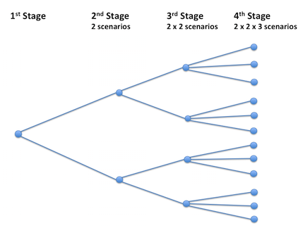
Note that the structure of the scenario tree is limited: each node in a stage has exactly the same number of arcs.
If there is more than one random variable per stage, then the number of scenarios increases accordingly. Note that there is no absolute limit to the number of stages and random variables, but the model can become very large very quickly as the number of stages and random variables increases. Note further that the random variables are stagewise independent. The realization of the random variables in one stage does not influence the realization of the random variables in a later stage.
Sampling Procedures
DE can solve only stochastic programs with random variables that follow discrete probability distributions. If the random data follows a continuous probability distribution the set \( \Omega \) has an infinite number of elements. Sampling is a process that generates a finite approximation \( \Omega_N \) to \( \Omega \). The size of \( \Omega_N \) is \(N\) and each element of \( \Omega_N \) has the same probability \( p=\frac{1}{N} \). Thus continuous probability distributions are approximated by discrete distributions. EMP SP provides the keyword sample to facilitate sampling. An example follows.
randvar d normal 45 10
sample d 100
These two lines are a portion of the emp.info file. In the first line d is defined as a random variable that follows a Normal distribution with mean 45 and standard deviation 10. In the second line it is specified that the continuous distribution is approximated by a sample of size 100. Note that the user determines the sample size \(N\). Note further that the use of the keyword sample is mandatory for random variables with continuous distributions. Otherwise the following error message will appear:
*** Only random variables with sampled continuous distributions supported.
Observe that behind the scenes the sampling is performed by the LINDO system. So the modeler needs a LINDO license for sample sizes larger than 10 (smaller sample sizes are included in the demo version). The LINDO system offers three variance reduction algorithms: the Antithetic algorithm, the Latin Square algorithm and the Monte Carlo algorithm. They may be enabled using either the option svr_ls_antithetic or svr_ls_latinsquare or svr_ls_montecarlo respectively.
Alternatively, the modeler may chose to generate a sample of the distribution first and then enter the sample as a discrete distribution in the emp.info file. There are two stochastic libraries that can be used for this procedure: the GAMS Stochastic Library and the LINDO Sampling Library. An example and details about the procedure using the LINDO library are given in section Sampling in the EMP manual.
The Expected Value Problem
Consider the special case where the sample size is 1 and the "sampled" value equals the expected value of the random variable. This entails that the random variable is replaced by its expected value. The resulting model is deterministic and is called the Expecetd Value Program. DE facilitates solving the Expected Value Problem through the option solveEVProb. If this option is specified in the option file (see example below) the Expected Value Problem is solved after the original stochastic model and the solution is reported. In addition, DE offers the option to choose a separate subsolver for the Expecetd Value Problem, the option evsubsolver.
In the following example the stochastic model is solved with the subsolver Conopt and the Expected Value Problem is solved with the subsolver Minos.
$onecho > de.opt
subsolver conopt
solveEVProb
evsubsolver minos
$offecho
mymodel.optfile=1;
solve mymodel min obj using emp scenario dict;
Note that the option solveEVProb is not defined for models with chance constraints and models featuring VaR and CVaR. These model types are discussed in the next section.
What types of models can DE handle?
As mentioned earlier, DE can solve two-stage and multi-stage stochastic linear, quadratic and nonlinear models and the mixed-integer versions of all these models. There are two further classes of stochastic models that DE is equipped to solve: stochastic programs with chance constraints and stochastic programs with other risk measures such as Variance at Risk (VaR) and Conditional Variance at Risk (CVaR). CVaR is also called Expected Shortfall.
In stochastic programs with chance constraints the goal is to make an optimal decision prior to the realization of random data while allowing the constraints to be violated with a certain probability. Mathematically, a stochastic linear program with chance constraints can be expressed as follows:
\begin{equation} \begin{array}{ll} \textrm{Min}_{x} & c^T x \\ \textrm{s.t.} & P(A x \leq b) \geq p\\ & x \geq 0,\\ \end{array} \end{equation}
where \( x \in \mathbb{R}^n \) is the decision variable and \( c^T \) denotes the coefficients of the objective function, \( A \in \mathbb{R}^{m \times n} \) is a random matrix and represents the coefficients and \( b \in \mathbb{R}^m \) is a random vector and denotes the right-hand side of the constraints. The distinctive feature of stochastic programs with chance constraints is that the constraints (or some of them) may be violated with probability \( \epsilon = 1-p \), where \(0 < p \leq 1\).
DE offers three reformulation options to solve stochastic programs with chance constraints: a reformulation using a mixed-integer program with big \( M \) notation, a convex hull reformulation and the use of indicator variables and indicator constraints. Note that the default is the MIP reformulation (the default value of \( M \) is set to 10000 and can be customized). With the option ccreform the reformulation method can be determined by the user.
For details on single and joint chance constraints and examples how to use the option ccreform, see the section Chance Constraints with EMP in the EMP manual. Note that random variables in programs with chance constraints may follow discrete or continuous probability distributions. Note further that there are no stages in stochastic programs with chance constraints.
As mentioned earlier, DE automatically optimizes the expected value of the objective function variable. DE also supports other risk measures, such as VaR and CVaR. In mathematical terms, DE is able to solve the following:
\begin{equation} \begin{array}{ll} \textrm{Min}_{x} & \mathcal{R} (z), \\ \end{array} \end{equation}
where \( z \) represents the objective function variable and \( \mathcal{R} \) denotes a risk measure such as the Expected Value, VaR and CVaR or a combination of risk measures (e.g. the weighted sum of Expected Value and CVaR). In addition, the modeler can also choose to trade off risk measures. For more details about risk measures see section Risk Measures with EMP in the EMP manual.
Reformulation Techniques
In this section some details are given about the reformulations that DE is performing behind the scenes.
Simple two-stage stochastic model
As mentioned previously, DE converts a stochastic model into its deterministic equivalent. Using the model nbsimple.gms from the GAMS EMP model library as an example, we show how exactly the deterministic equivalent is built. Note that this model is also discussed in detail in the section A Simple Example: The News Vendor Problem of the EMP manual.
The model is given by the following equations:
\begin{equation} \textrm{Max}_{x} \quad z(x) = - cx + \mathbb{E}[Q(x,\omega)], \quad x\geq 0, \end{equation}
where
\begin{align} Q(x,\omega) = & \, \textrm{Max}_{s, i, l} \qquad \, vs(\omega) - hi(\omega) -pl(\omega) \nonumber \\ &\, \textrm{s.t.} \qquad \, \, \, x - \, \, s(\omega) - \, \, i(\omega) \quad \quad \qquad \, = \, 0 \nonumber \\ &\, \qquad \quad \quad \qquad \, \, s(\omega) \qquad \quad \quad \, + \, l(\omega) \, = \, d(\omega) \nonumber \\ &\qquad \qquad \quad \quad \, \, s(\omega), \, i(\omega), \, l(\omega) \, \geq 0 \quad \forall \omega \in \Omega. \nonumber \end{align}
Here \(c\), \(v\), \(h\) and \(p\) are some given parameters, the first-stage decision variable is \(x\), the second-stage decision variables are \(s\), \(i\) and \(l\) and the uncertain data is represented by the random variable \(d(\omega)\). We assume that the annotations specify that \(d\) follows a Normal distribution and the sample size to approximate this continuous distribution is 4 (where all scenarios are equally likely, so \(p(s) = 0.25\)).
First, DE draws 4 values from the Normal distribution specified in the annotations. These 4 values are the basis for the 4 scenarios that are generated. For each scenario, a separate equation for the two second-stage constraints is built (that are 8 equations). In the process, for each of the three decision variables of the second stage 4 variables are generated since the second-stage decision variables may take different values for each scenario. Next, an equation for the profit for each scenario is generated (4 equations) and finally, the equation to compute the average profit is built. So there are a total of 13 equations. They are given here:
\begin{equation} \begin{array}{lll} x - s_1 - i_1 & = & 0 \\ x - s_2 - i_2 & = & 0 \\ x - s_3 - i_3 & = & 0 \\ x - s_4 - i_4 & = & 0 \\ s_1 + l_1 & = & d_1 \\ s_2 + l_2 & = & d_2 \\ s_3 + l_3 & = & d_3 \\ s_4 + l_4 & = & d_4 \\ z_1 & = & -cx + vs_1 - hi_1 - pl_1 \\ z_2 & = & -cx + vs_2 - hi_2 - pl_2 \\ z_3 & = & -cx + vs_3 - hi_3 - pl_3 \\ z_4 & = & -cx + vs_4 - hi_4 - pl_4 \\ z & = & 0.25 z_1 + 0.25 z_2 + 0.25 z_3 + 0.25 z_4 \\ \end{array} \end{equation}
Note that there is only one realization of the first-stage decision variable \(x\) while for the second-stage decision variables there as many realizations as there are scenarios.
A multi-stage stochastic model
DE recursively builds a scenario tree to generate the deterministic equivalent of multi-stage models. We take the model inventory from the EMP manual to demonstrate how this is done. The 4-stage model is given by the following equations:
\begin{align} \textrm{Max}_{y_1, i_1} \quad & z = - \alpha y_1 -\gamma i_1 + \mathbb{E}[ Q( (y_1,i_1), \omega_{\text{I}}) + \mathbb{E}[ Q( (y_1,i_1), \omega_{\text{II}}) + \mathbb{E}[ Q( (y_1,i_1), \omega_{\text{III}}) ]]] \nonumber \\ \textrm{s.t.} \quad \qquad & i_1 = y_1 \nonumber \\ & y_1, i_1 \geq 0, \nonumber \end{align}
where
\begin{align} Q((y_1,i_1), \omega_{\zeta}) = \, \textrm{Max}_{s_t, y_t, i_t} \, & \beta s_t(\omega_{\zeta}) - \alpha y_t(\omega_{\zeta}) - \delta i_t(\omega_{\zeta}) \nonumber \\ \textrm{s.t.} \quad \quad \quad & i_{t-1} + y_t = s_t + i_t \nonumber \\ & s_t \leq i_{t-1} \nonumber \\ & s_t \leq d_t(\omega_{\zeta}) \nonumber \\ & i_t \leq \kappa \nonumber \\ & s_t, y_t, i_t \geq 0 \quad \textrm{for} \quad t = 2,3,4. \nonumber \end{align}
Here \(y_1\) and \(i_1\) are the first-stage decision variables and \(y_t\), \(i_t\) and \(s_t\) are the decision variables of the later stages; \(\alpha\), \(\beta\), \(\gamma\), \(\delta\) and \(\kappa\) denote fixed parameters. The uncertain data is represented by the random variable \(d_t(\omega_{\zeta})\), where \(\omega_{\zeta} \in \Omega_{\zeta}\) and \(\zeta = \text{I}, \text{II}, \text{III}\). Note that \(s_t\), \(y_t\) and \(i_t\) depend on the realization of \(d_t\). Now assume that \(d_t\) follows a continuous distribution and the sample size to approximate this distribution is just 3 for stages 2 to 4. Note that in multi-stage models the sample size may vary for each stage. Note further that for all practical purposes this sample size is too small, it was chosen here for reasons of clarity of exposition. As usual, the distribution(s) and sample size(s) are specified in the annotations. Observe that the last constraint ( \( i_t \leq \kappa \)) is implemented as a bound on the variable \(i_t\), not as an equation. So, in addition to the objective equations, there is one equation in the first stage and three equations in each of the later stages.
This model is reformulated in the following way. First, an equation for the first stage constraint is generated. Secondly, three realizations of \(d_2\) are chosen through a sampling procedure, so there are three scenarios at stage 2. For each of these three realizations of the random variable the equations for the second stage are generated (9 equations). Thirdly, three realizations of \(d_3\) are sampled for stage 3. Each of these three realizations may follow one of the three scenarios of the second stage, so there are nine scenarios in stage 3 and hence \(9 \times 3 = 27\) equations are generated for stage 3. The procedure is repeated in stage 4 where there are 27 scenarios and \( 27 \times 3 = 81 \) equations. Next, the value of the objective variable for each scenario is computed by generating 27 equations for \(z_s\) and finally, an equation to compute \(z\) is built, where \( z = \sum_s p(s) z_s \).
Chance Constraints
Models with chance constraints are reformulated as mixed integer problems by default. This reformulation is discussed in detail in the section Chance Constraints with EMP in the EMP manual. Reformulations using a convex hull or indicator variables and indicator constraints are also possible. The reformulation method may be determined by the user with the option ccreform.
Computing VaR
Models involving VaR are reformulated using mixed integer programs with big \(M\) notation. By the example model portfolio.gms we demonstrate how this is done. This model is discussed in the section Value at Risk (VaR) in the EMP manual. The model is given by the following equations:
\begin{equation} \begin{array}{ll} \textrm{Max} & \underline{VaR}_{\theta}[R] \\ \textrm{s.t} & R = \sum_j w_j v_j(\omega) \qquad \forall \omega \in \Omega\\ & \sum_j w_j = 1 \\ & w_j \geq 0,\\ \end{array} \end{equation}
where \(\underline{VaR}_{\theta}\) is the VaR at the lower \(\theta\)th percentile, the variable \(R\) is the return (and is a function of the random variable \(v_j(\omega)\)), \(w_j\) the weight associated with each asset \(j\) and \(v_j(\omega)\) is the (random variable) return of each asset \(j\). The weights can also be interpreted as proportions of the amount to be invested, their sum must be 1. Note that \(w_j\) is the decision variable in this problem.
Let \( y(s) \) be a binary variable that acts as an indicator variable. For each scenario, it equals 1 if the return \( R \geq \underline{VaR}_{\theta}[R] \) and it is 0 otherwise. Then the model is reformulated to the following MIP:
\begin{equation} \begin{array}{ll} \textrm{Max} & \underline{VaR}_{\theta}[R] \\ \textrm{s.t} & r(s) = \sum_j w_j v_j(s) \qquad \qquad \qquad \qquad \forall s = 1, \dots , S \\ & r(s) \geq \underline{VaR}_{\theta}[R] - M (1-y(s)) \quad \quad \forall s = 1, \dots , S \\ & cc = 1- \sum_s p(s)y(s) \\ & \sum_j w_j = 1 \\ & 0 \leq cc \leq \theta \\ & w_j \geq 0.\\ \end{array} \end{equation}
Here \( r(s) \) denotes the return per scenario and \( cc \) is a variable that represents the probability of violations (a violation occurs if in a scenario the return is smaller than \( \underline{VaR}_{\theta}[R] \)). As usual, \( p(s) \) is the probability that a scenario occurs and \( M \) is the big \( M \). The first three constraints together with the bounds on \( cc \) ensure that the probability of violations is smaller than or equal to \( \theta \).
Note that the default value for big \(M\) for models with VaR is 1000 (and it is different from the default value for big \(M\) for chance constraints). It may be customized with the option varbigm.
Computing CVaR
Models with CVaR are reformulated by converting the annotations into new variables and equations. Using the model portfolio.gms as an example we demonstrate how this is done. This model features in the GAMS EMP library and is also discussed in the section Conditional Value at Risk (CVaR) in the EMP manual. The model is given by:
\begin{equation} \begin{array}{ll} \textrm{Max} & \underline{CVaR}_{\theta}[R] \\ \textrm{s.t} & R = \sum_j w_j v_j(\omega) \qquad \forall \omega \in \Omega\\ & \sum_j w_j = 1 \\ & w_j \geq 0,\\ \end{array} \end{equation}
where \(\underline{CVaR}_{\theta}\) is the CVaR at the left tail of the distribution at the confidence level \(\theta\) and all other variables are as defined above. Note that again, \(w_j\) is the decision variable in this problem.
DE reformulates this model by introducing three new variables and three associated equations. Let \(r(s)\) denote the return per scenario, \(t\) the target return to be achieved with probability approximately \(1-\theta\) and \(d(s)\), \(d(s) \geq 0\), the lower deviation from \(t\) per scenario. The equations follow.
\begin{equation} \begin{aligned} r(s) & = \sum_j w_j v_j(s) \\ d(s) & \geq t - r(s) \\ \underline{CVaR}_{\theta}[R] & = t - \frac{1}{\theta} \sum p(s) d(s) \end{aligned} \end{equation}
Thus the model is reformulated to an LP and may be solved by an appropriate solver. It is easy to see that \(t\) equals \( \underline{VaR}_{\theta}[R] \).
Logfile
The logfile gives much information about the solver progress. The following is the DE log output from running the nbdiscjoint model from the GAMS EMP Model Library:
--- Starting compilation
--- nbdisjoint.gms(74) 3 Mb
--- Starting execution: elapsed 0:00:00.024
--- nbdisjoint.gms(72) 4 Mb
---
--- collecting and writing gdx file
---
--- Generating EMP model nb
--- nbdisjoint.gms(72) 6 Mb
---   5 rows  9 columns  19 non-zeroes
---   6 nl-code  2 nl-non-zeroes
--- nbdisjoint.gms(72) 4 Mb
--- Executing DE: elapsed 0:00:00.083
--- Input model type identified and solved as LP
DE               24.5.1 r54187 Released Sep 23, 2015 DEG x86 64bit/MacOS X
--- DE has 26 rows 50 columns 116 non-zeroes

IBM ILOG CPLEX   24.5.1 r54187 Released Sep 23, 2015 DEG x86 64bit/MacOS X
Cplex 12.6.2.0

Reading data...
Starting Cplex...
Unable to load names.
Tried aggregator 1 time.
LP Presolve eliminated 14 rows and 31 columns.
Reduced LP has 12 rows, 19 columns, and 36 nonzeros.
Presolve time = 0.01 sec. (0.02 ticks)

Iteration log . . .
Iteration:     1   Dual infeasibility =            52.800000
Iteration:    10   Dual objective     =          2660.700000
LP status(1): optimal
Cplex Time: 0.06sec (det. 0.05 ticks)

Optimal solution found.
Objective :        1173.900000

--- Restarting execution
--- nbdisjoint.gms(72) 2 Mb
--- Reading solution for model nb
--- nbdisjoint.gms(72) 3 Mb
---
--- scattering and reading gdx file
---
--- randvar  Id = d maps to s_d
--- nbdisjoint.gms(72) 3 Mb
--- randvar  Id = r maps to s_r
--- level    Id = s maps to s_s
--- level    Id = x maps to s_x
--- nbdisjoint.gms(72) 4 Mb
--- Scatter finished in 2 ms
--- nbdisjoint.gms(74) 4 Mb
*** Status: Normal completion
--- Job nbdisjoint.gms Stop 12/06/15 18:02:47 elapsed 0:00:00.382
First, the model in scalar form is generated. It has 5 equations, so the model statistics report 5 rows. Further, it has 6 positive variables, one free variable and 2 random variables, so there are 9 columns. A matrix form representation of the model with the variables as columns and the equations as rows has 19 non-zero entries. Next, DE generates the deterministic equivalent. The statistics for the deterministic equivalent indicate that there are 26 rows, 50 columns and 116 non-zero entries. The stochastic model has 6 scenarios, so for each second-stage equation there are 6 equations in the deterministic equivalent (i.e. a total of 24 equations). In addition, there is one first-stage equation and one equation to compute the expected value of the objective variable, which brings the sum total to 26 equations or rows. Similarly, for each second-stage variable in the stochastic model there are 6 variables in the determininistic equivalent (i.e a total of 48 variables). In addition, there is the first-stage decision variable and a variable for the expected value of the objective adding up to a total of 50 variables or columns.
Note that the model type is identified as an LP and thus the default LP solver is invoked. In this case the subsolver is Cplex and most of the remainder of the logfile is output from the subsolver. At the end the mapping specified in the dictionary is performed.
The logfile of solving stochastic models with VaR or CVaR is similar. It reports that the model type is being determined, the deterministic equivalent built and then handed over to the appropriate subsolver to be solved. However, when solving stochastic programs with chance constraints there is much more happening behind the scenes. DE automatically hands over the model to the subsolver JAMS. By default, JAMS reformulates the model and generates a scalar version of it. The scalar version of the reformulated model is then handed back to the GAMS system to be solved by an appropriate subsolver. The logfile reports the progress of the subsolver until the model is solved. Then the solution from the GAMS subsolver is handed to JAMS and a list of disjunctions and their activity level is reported. (The equations in the scalar version of the reformulated model that may be left unsatisfied are called disjunctions. Active disjunctions refer to equations that are satisfied and not active disjunctions refer to equations that are not satisfied.)
Parts of the DE logfile from running the simplechance model from the GAMS EMP Model Library are given below. These parts of the logfile demonstrate the solution process for stochastic models with chance constraints that was just described.
...
--- Generating EMP model sc
--- simplechance.gms(79) 6 Mb
---   3 rows  5 columns  9 non-zeroes
---   9 nl-code  4 nl-non-zeroes
--- simplechance.gms(79) 4 Mb
--- Executing DE: elapsed 0:00:00.024
--- Input model type identified and solved as LP
DE               24.5.1 r54187 Released Sep 23, 2015 DEG x86 64bit/MacOS X

--- Reset Solvelink = 2

JAMS 1.0         24.5.1 r54187 Released Sep 23, 2015 DEG x86 64bit/MacOS X

JAMS - Solver for Extended Mathematical Programs (EMP)
------------------------------------------------------

--- Using Option File
Reading parameter(s) from "jams.159"
>>  EMPInfoFile .../Models/225a/jamsinfo.dat
>>  SubSolver CPLEX
Finished reading from "jams.159"

--- EMP Summary
    Logical Constraints = 0
    Disjunctions        = 7
    Adjusted Constraint = 0
    Flipped Constraints = 0
    Dual Variable Maps  = 0
    Dual Equation Maps  = 0
    VI Functions        = 0
    Equilibrium Agent   = 0
    Bilevel Followers   = 0

*** Warning 7 of 7 BigM disjunctions use DE's default for bigM (10000)

--- The model .../Models/225a/emp.dat will be solved by GAMS
---
--- Job emp.dat Start 12/06/15 18:43:18 24.5.1 r54187 DEX-DEG x86 64bit/MacOS X
GAMS 24.5.1   Copyright (C) 1987-2015 GAMS Development. All rights reserved
...
--- Generating MIP model m
--- emp.dat(68) 3 Mb
---   10 rows  19 columns  40 non-zeroes
---   7 discrete-columns
--- Executing CPLEX: elapsed 0:00:00.016

IBM ILOG CPLEX   24.5.1 r54187 Released Sep 23, 2015 DEG x86 64bit/MacOS X
Cplex 12.6.2.0

Reading data...
Starting Cplex...
....
MIP Solution:            4.750000    (11 iterations, 0 nodes)
Final Solve:             4.750000    (2 iterations)
...
--- Reading solution for model m
*** Status: Normal completion
--- Job emp.dat Stop 12/06/15 18:43:18 elapsed 0:00:00.299
--- Returning from GAMS step
---
--- Disjunction Summary
    Disjunction 1 is not active
    Disjunction 2 is active
    Disjunction 3 is active
    Disjunction 4 is active
    Disjunction 5 is not active
    Disjunction 6 is active
    Disjunction 7 is active
---
--- Restarting execution
--- simplechance.gms(79) 2 Mb
--- Reading solution for model sc
--- simplechance.gms(79) 3 Mb
---
--- scattering and reading gdx file
---
--- randvar  Id = om1 maps to s_om1
--- simplechance.gms(79) 3 Mb
--- randvar  Id = om2 maps to s_om2
--- level    Id = x1 maps to x1_l
--- marginal Id = x1 maps to x1_m
--- level    Id = x2 maps to x2_l
--- level    Id = e1 maps to e1_l
--- level    Id = e2 maps to e2_l
--- simplechance.gms(79) 4 Mb
--- Scatter finished in 2 ms
--- simplechance.gms(81) 4 Mb
*** Status: Normal completion
Summary of DE Options
General Options
| Option | Description | Default |
|---|---|---|
| correlationtype | Sample correlation type | 0 |
| empinfofile | Path and name of file containing additional EMP-SP information as randvar, jrandvar, stage etc. | |
| subsolver | Subsolver to run | |
| subsolveropt | Optfile value to pass to the subsolver | 1 |
| svr_ls_antithetic | Sample variance reduction map to Lindo Antithetic algorithm | |
| svr_ls_latinsquare | Sample variance reduction map to Lindo Latin Square algorithm | |
| svr_ls_montecarlo | Sample variance reduction map to Lindo Montecarlo algorithm |
Options for chance constraint models
| Option | Description | Default |
|---|---|---|
| ccreform | Reformulation option passed to JAMS | bigM |
| jamsopt | JAMS option file |
Options for recourse models
| Option | Description | Default |
|---|---|---|
| evsubsolver | Subsolver to run on expected value problem | |
| evsubsolveropt | Optfile value to pass to the subsolver for expected value problem | 1 |
| maxnodes | Tree size limit | 100000 |
| solveEVProb | Solve and report the expected value solution | 0 |
| varbigm | Big M for Value at Risk reformulation | 1000.0 |
Detailed Descriptions of DE Options
ccreform (string): Reformulation option passed to JAMS ↵
This option determines how to formulate the indicator contraints of the chance constraints in the deterministic equivalent. The model is passed to JAMS for the actual reformulation and solution with a subsolver. The possible reformulation options are
bigM [big eps threshold],chull [big eps], andindic. Theindicsetting only works with solver that under stand the indicator syntax in a GAMS option file.Default:
bigM
correlationtype (integer): Sample correlation type ↵
Default:
0
value meaning 0Pearson 1Kendall 2Spearman
empinfofile (string): Path and name of file containing additional EMP-SP information as randvar, jrandvar, stage etc. ↵
evsubsolver (string): Subsolver to run on expected value problem ↵
evsubsolveropt (integer): Optfile value to pass to the subsolver for expected value problem ↵
Range: {
1, ...,999}Default:
1
jamsopt (string): JAMS option file ↵
maxnodes (integer): Tree size limit ↵
Range: {
1000, ..., ∞}Default:
100000
solveEVProb (no value): Solve and report the expected value solution ↵
Default:
0
subsolver (string): Subsolver to run ↵
subsolveropt (integer): Optfile value to pass to the subsolver ↵
Range: {
1, ...,999}Default:
1
svr_ls_antithetic (string): Sample variance reduction map to Lindo Antithetic algorithm ↵
svr_ls_latinsquare (string): Sample variance reduction map to Lindo Latin Square algorithm ↵
svr_ls_montecarlo (string): Sample variance reduction map to Lindo Montecarlo algorithm ↵
varbigm (real): Big M for Value at Risk reformulation ↵
Default:
1000.0